Connecting Vision and Language: A Deep Dive into OpenAI’s CLIP

A detailed breakdown of the paper that taught a computer to see the world through the lens of human language, enabling remarkable zero shot image classification.

For years, the gold standard in computer vision involved training models on massive, manually labeled datasets like ImageNet. While incredibly successful, this approach has a fundamental limitation: the model’s knowledge is confined to the specific categories it was trained on. In a parallel revolution, natural language processing (NLP) models like GPT-3 moved towards pre-training on the vast, raw text of the internet, learning flexible and generalizable knowledge. The OpenAI CLIP paper asks a powerful question: can we bring the NLP pre-training paradigm to computer vision and learn from the rich, descriptive text that naturally accompanies images online?

Abstract

The Problem: The “Fixed Set” Limitation of Vision Models

The authors start by highlighting a long-standing challenge in computer vision.

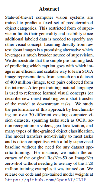
State-of-the-art computer vision systems are trained to predict a fixed set of predetermined object categories. This restricted form of supervision limits their generality and usability since additional labeled data is needed to specify any other visual concept.

For years, the standard approach was to train a model on a dataset with a predefined list of categories, like the 1000 object classes in the famous ImageNet dataset. If a model was trained to recognize “cats,” “dogs,” and “cars,” it had no inherent ability to recognize a “horse” or a “bicycle.” To teach it a new concept, you had to go back, collect and label thousands of new images, and fine-tune or retrain the model. This process is expensive, slow, and fundamentally limits a model’s real world usefulness. The world is not a fixed set of 1000 categories.

The Solution: Learning from Natural Language

Instead of relying on these rigid, curated datasets, the authors propose a more natural and scalable alternative.

Learning directly from raw text about images is a promising alternative which leverages a much broader source of supervision. We demonstrate that the simple pre-training task of predicting which caption goes with which image is an efficient and scalable way to learn SOTA image representations from scratch on a dataset of 400 million (image, text) pairs collected from the internet.

This is the core idea of CLIP. The internet is filled with images, and those images are often paired with descriptive text: captions, articles, titles, etc. This text provides a rich source of information, or what the authors call supervision. Instead of teaching a model that an image maps to a single label like dog, we can teach it that an image maps to a descriptive phrase like "a photo of a golden retriever playing in the park".

By training on a massive, custom-built dataset of 400 million of these (image, text) pairs, the model learns a much more nuanced and flexible understanding of visual concepts. The goal of the training is simple: given a batch of images and a batch of captions, the model must figure out which caption correctly describes which image.

The Payoff: True Zero-Shot Transfer

This training approach unlocks the model’s most powerful capability.

After pre-training, natural language is used to reference learned visual concepts (or describe new ones) enabling zero-shot transfer of the model to downstream tasks.

Because CLIP learns to connect the content of an image to the meaning of text, you can now give it classification tasks it has never seen before, simply by describing the classes in plain English. This is called zero-shot transfer.

Imagine you want to classify photos of different dog breeds. With a traditional model, you’d need a labeled dataset of thousands of dog photos. With CLIP, you simply provide the text descriptions, like "a photo of a golden retriever", "a photo of a poodle", "a photo of a husky", and the model can instantly classify images into these new categories without seeing a single labeled example. It’s using its pre-trained knowledge to connect what it “sees” in the image to the text you provide.

The Evidence: It Actually Works

The authors back up this powerful claim with extensive testing.

We study the performance of this approach by benchmarking on over 30 different existing computer vision datasets… For instance, we match the accuracy of the original ResNet-50 on ImageNet zero-shot without needing to use any of the 1.28 million training examples it was trained on.

This is the headline result. They tested CLIP’s zero-shot performance across a huge range of tasks, from recognizing objects and actions to reading text (OCR). The most stunning demonstration is its performance on ImageNet. Without being trained on any of the 1.28 million ImageNet training images, CLIP was able to match the accuracy of a fully-supervised ResNet-50 model that was explicitly trained on that data. This proves that learning from natural language supervision is not just a clever idea, but a highly effective method for building general-purpose visual models.

TipA Quick Note: How Does CLIP Actually Classify an Image?

One of the most profound ideas in the CLIP paper is that the model does not have a fixed list of categories it can recognize. This is a radical departure from how most computer vision models worked before it. To truly appreciate this, let’s compare the traditional approach to CLIP’s new paradigm.

The Traditional Approach: A Built-in Classifier

Think of a classic image classification model like a ResNet-50 trained on the ImageNet dataset. Its architecture is typically composed of two main parts:

1. Feature Extractor: A deep stack of convolutional layers that process an input image and convert it into a high level feature representation (essentially, a vector or list of numbers).
2. Classifier Head: A final, fully connected layer at the very end of the network. For a model trained on ImageNet, this layer has exactly 1000 outputs, one for each of the 1000 specific classes in the dataset.

The model is trained to make the output corresponding to the correct class have the highest score. This structure is rigid. The model can only ever predict one of the 1000 classes it was explicitly built to recognize. If you want it to recognize a new object, you have to replace or retrain this final layer.

The CLIP Approach: A Dynamic Classifier from Language

CLIP gets rid of the fixed classifier head entirely. Instead, it learns a shared space where both images and text can coexist. It does this using two separate encoders:

1. Image Encoder: Takes an image and turns it into a feature vector.
2. Text Encoder: Takes a piece of text (a word, a phrase, or a sentence) and turns it into a feature vector.

The key is that both models are trained together to place the vectors for a matching (image, text) pair as close as possible in this shared space, which we can call a “multimodal embedding space”. Think of it as a universal “concept space” where visual and textual ideas that mean the same thing are placed near each other.

So, when you ask CLIP to perform a classification task, here is what happens behind the scenes:

1. Step 1: Encode the Image. You feed a single image (for instance, a photo of a cat) into CLIP’s Image Encoder. The output is a single vector that numerically represents the content of the image.
2. Step 2: Encode the Potential Classes. You create a list of text descriptions for all your target classes. For example: "a photo of a dog", "a photo of a car", "a photo of a cat". You then feed this list into CLIP’s Text Encoder. The output is a set of vectors, one for each text description.
3. Step 3: Find the Best Match. CLIP then calculates the similarity (specifically, the cosine similarity) between the one image vector and every single one of the text vectors.
4. Step 4: Make the Prediction. The text description whose vector is most similar to the image vector is the model’s prediction. In our example, the vector for "a photo of a cat" would be “closest” to the image vector, making that the final classification.

The “classifier” is not a static part of the model’s architecture; it is something you create dynamically at inference time just by providing text. This is what gives CLIP its incredible flexibility. You can swap out your list of classes for any other visual concept you can describe with words, all without retraining the model. This is the essence of its powerful zero shot capability.

1. Introduction and Motivating Work

The NLP Revolution: A Blueprint for Vision

To understand the genius of CLIP, we first have to look away from computer vision and towards its sister field, Natural Language Processing. The authors of CLIP didn’t invent their core strategy from scratch; they brilliantly adapted a paradigm that had already proven phenomenally successful in the world of text.

Pre-training methods which learn directly from raw text have revolutionized NLP over the last few years (Dai & Le, 2015; Peters et al., 2018; Howard & Ruder, 2018; Radford et al., 2018; Devlin et al., 2018; Raffel et al., 2019).

The authors are referencing a seismic shift in NLP. Before this “revolution,” NLP models were often trained for a specific task (e.g., sentiment analysis) on a relatively small, task specific dataset. The breakthrough was the idea of pre-training: first, train a massive model on a gigantic corpus of raw, unlabeled text from the internet. The goal wasn’t to perform a specific task, but to learn the underlying patterns, grammar, and concepts of language itself. This pre-trained model could then be quickly adapted (or “fine-tuned”) for specific tasks with much less data and achieve state of the art results.

Task-agnostic objectives such as autoregressive and masked language modeling have scaled across many orders of magnitude in compute, model capacity, and data, steadily improving capabilities.

This sentence explains how this pre-training works. Since you don’t have explicit labels, you need a “self-supervised” or task-agnostic objective. This means the learning task is generated from the data itself, not from human labels. The two most famous objectives are:

• Autoregressive Language Modeling: This simply means “predicting the next word.” The model is given a sequence of text like “The cat sat on the” and its goal is to predict the next word, “mat”. This is the fundamental principle behind models like GPT (Generative Pre-trained Transformer).
• Masked Language Modeling (MLM): Instead of just predicting the next word, this approach takes a sentence, masks out a word (e.g., “The cat [MASK] on the mat”), and tasks the model with predicting the missing word. This forces the model to learn context from both the left and the right, and it’s the core idea behind the hugely influential BERT model.

These simple, scalable objectives allowed researchers to throw massive amounts of data and compute at their models, leading to rapid improvements.

The development of “text-to-text” as a standardized input-output interface … has enabled task-agnostic architectures to zero-shot transfer to downstream datasets removing the need for specialized output heads or dataset specific customization. Flagship systems like GPT-3 … are now competitive across many tasks with bespoke models while requiring little to no dataset specific training data.

This is the ultimate payoff of the NLP paradigm. By framing every problem as a “text-in, text-out” task, models became incredibly flexible. For example, instead of training a specialized translation model, you could just feed a model like Google’s T5 the text: "translate English to German: Hello, how are you?" and it would learn to output: "Hallo, wie geht es Ihnen?".

This flexibility, supercharged by massive scale, led to models like GPT-3. GPT-3 is a single, pre-trained model that can perform a staggering variety of tasks it was never explicitly trained for (summarization, coding, creative writing, classification) simply by being given the right text prompt. It doesn’t need specialized “output heads” (like the fixed classifier layers we discussed earlier) and requires little to no task specific training data.

In essence, the authors are setting the stage by saying: “Look at the incredible power and flexibility NLP unlocked by moving from small, labeled datasets to massive, self-supervised pre-training. We are going to do the same thing for computer vision.”

TipGPT-3 vs. T5: Two Philosophies of Language Modeling

While both are massive Transformer-based models pre-trained on web-scale text, GPT-3 and T5 are built on different fundamental principles that make them better suited for different kinds of tasks.

At a high level, you can think of the difference with this analogy:

• GPT-3 is a brilliant autocomplete. It is an expert at continuing a piece of text. Its core strength is open-ended generation.
• T5 is a universal translator. It is an expert at transforming an input text into a desired output text. Its core strength is transformation and structured tasks.

Let’s look at the key technical differences that lead to this behavior.

1. Training Objective: The Core Task

This is the most important distinction.

• GPT-3 (Autoregressive): As we discussed, GPT-3 is trained on an autoregressive objective, which simply means “predict the next word.” It reads text from left to right and learns to predict the most probable next token given the preceding context. It never sees “the future”; it only ever looks backward.

• T5 (Text-to-Text Denoising): T5 (Text-to-Text Transfer Transformer) is trained on a “fill-in-the-blank” objective, inspired by BERT’s Masked Language Modeling. During pre-training, it takes a clean sentence, randomly “corrupts” it by masking out spans of text, and is then asked to reconstruct the original, uncorrupted text.

  For example:

  • Original: Thank you for inviting me to the party last week.
  • Corrupted Input to T5: Thank you <X> me to the party <Y> week.
  • T5’s Target Output: <X> for inviting <Y> last

  This “denoising” objective forces the model to become very good at understanding the full context of a sentence to fill in the missing parts. This makes it a natural fit for tasks that require transforming an input into an output.

2. Model Architecture

Their training objectives lead to different choices in the underlying Transformer architecture.

• GPT-3 (Decoder-Only): Because its only job is to generate the next word based on past context, GPT-3 uses only the decoder blocks from the original Transformer architecture. The decoder’s “masked self-attention” mechanism is perfectly suited for this, as it ensures that when predicting a word, the model can only attend to the words that came before it.

• T5 (Encoder-Decoder): T5 uses the full encoder-decoder architecture from the original Transformer.

  • The Encoder reads the entire corrupted input sequence at once (e.g., Thank you <X> me to the party...). This allows it to build a complete, bidirectional understanding of the context.
  • The Decoder then takes the encoder’s representation and generates the target output (e.g., <X> for inviting...) in an autoregressive, word-by-word fashion. This structure is ideal for sequence-to-sequence tasks like translation and summarization.

3. Typical Use Case

Their design differences make them shine in different scenarios.

• GPT-3 is best for:
  • Open-ended generation: Creative writing, brainstorming, writing code, creating long-form content.
  • Few-shot prompting: Its massive scale gives it an incredible ability to perform tasks just by seeing a few examples in the prompt, without any retraining.
  • Chatbots and conversational AI.
• T5 is best for:
  • Transformation tasks: Summarization (long text in, short text out), translation (English in, German out), question answering (question in, answer out).
  • Fine-tuning: It serves as a powerful, general-purpose base model that is explicitly designed to be fine-tuned on specific datasets to become an expert at a particular transformation task.

Summary Table

Feature	GPT-3 (and GPT family)	T5 (and BERT-style models)
Primary Goal	Generation	Transformation
Training Objective	Autoregressive (Predict next word)	Denoising (Fill in the blanks)
Architecture	Decoder-Only	Encoder-Decoder
Data Flow	Unidirectional (looks at past context)	Bidirectional (looks at all context)
Best For	Creative writing, few-shot prompting	Summarization, translation, fine-tuning

The CLIP paper references the innovations from both of these camps. It takes the idea of massive scale and flexible, zero-shot transfer from the GPT world and applies it to a task that is conceptually more like a transformation (image in, text description out).

TipA Quick Note: If GPT is a “Next-Word Predictor,” How Can It Summarize?

This is a brilliant question that highlights a key development in modern AI. The base GPT-3 model is, at its core, an autoregressive, “next-word predictor.” In contrast, models like T5 are built with an encoder-decoder structure that is a more natural architectural fit for summarization. So how can ChatGPT, which is based on the GPT architecture, be so good at it?

The answer lies in two concepts: emergent abilities from scale and a powerful fine-tuning process called instruction tuning (and RLHF).

1. Emergent Abilities from Scale

A base GPT model is trained on a simple goal: predict the next word. But to get really good at this task across a dataset as vast and diverse as the internet, the model cannot simply memorize sequences. It is forced to build a deep, internal understanding of language and the world. It must learn:

• Grammar and Syntax: The rules of language.
• Semantic Concepts: The meaning of words and how they relate (e.g., that “king” - “man” + “woman” is close to “queen”).
• Factual Knowledge: Information about people, places, and events.
• Context and Cohesion: How sentences and paragraphs logically follow each other.

To accurately predict the next word of a complex article, the model must implicitly keep track of the article’s main topic and key points. In a sense, the ability to “understand” for the purpose of summarization is an emergent property that arises as a side effect of getting extremely good at next-word prediction at a massive scale.

The base model saw countless examples of articles followed by abstracts or summaries in its training data. So, if you prompt it correctly (e.g., by providing an article followed by TL;DR:), it recognizes this pattern and knows that the most probable “next words” are a condensed version of the preceding text. It’s completing a pattern it has learned.

2. Instruction Tuning and RLHF: The Secret Sauce of ChatGPT

This is the most critical factor. ChatGPT is not the base GPT-3 model. It is a variant that has gone through an extensive, second phase of training designed specifically to make it a helpful assistant.

This process involves two main steps:

• Instruction Tuning (Supervised Fine-Tuning): First, the base GPT model is fine-tuned on a high-quality, curated dataset of (instruction, desired_output) pairs. These were created by human labelers. For summarization, this dataset would contain thousands of examples like:

  Instruction: "Summarize the following scientific abstract for a fifth-grader: [long, complex abstract text]"

  Desired Output: "[simple, easy-to-understand summary]"

  By training on millions of such instructions across thousands of different tasks, the model learns to generalize the concept of following instructions, not just completing patterns.

• Reinforcement Learning from Human Feedback (RLHF): This is the step that truly refines the model’s behavior. In this stage, the model generates several different responses to a single prompt (e.g., four different summaries). A human rater then ranks these responses from best to worst. This feedback is used to train a separate “reward model.” Finally, the main GPT model is fine-tuned again using reinforcement learning to maximize the score it gets from this reward model.

In simple terms, RLHF trains the model to produce outputs that humans find helpful, accurate, and well-written.

The Bottom Line

You can think of it like this:

• Base GPT-3 is like a brilliant student who has read every book in the library. They have all the knowledge, but they are not trained to apply it to specific tasks for you. They might answer your question, or they might just continue your sentence in a creative but unhelpful way.
• ChatGPT is that same brilliant student after they have completed a rigorous apprenticeship on how to be the world’s best assistant. They have been explicitly trained to understand and follow instructions, including “summarize this,” making them far more reliable and useful for such tasks.

So, while T5’s architecture is a natural fit for summarization, ChatGPT’s massive scale and, more importantly, its specialized instruction-following and RLHF training give it the powerful ability to perform this and many other structured tasks exceptionally well.

The Central Question: Can Vision Learn from NLP’s Playbook?

After establishing the success of pre-training on raw web text in NLP, the authors pivot to make their main point: computer vision has not yet embraced this paradigm, and perhaps it should.

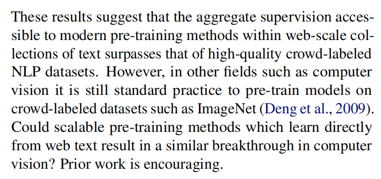
These results suggest that the aggregate supervision accessible to modern pre-training methods within web-scale collections of text surpasses that of high-quality crowd-labeled NLP datasets.

This is a powerful claim. The authors are arguing that the sheer volume and diversity of text on the internet (the “aggregate supervision”) is a more potent teacher than smaller, meticulously human-labeled datasets. Think of it this way: a “crowd-labeled” dataset might have thousands of perfectly annotated examples for a specific task like question answering. But the internet has trillions of words discussing nearly every topic imaginable, from cooking to quantum mechanics to celebrity gossip. The authors’ claim is that the raw breadth and variety of this web-scale data provides a richer, more generalizable learning signal than any clean, but narrow, dataset ever could. Quantity and variety have a quality all their own.

Having made this point about NLP, they immediately contrast it with computer vision:

However, in other fields such as computer vision it is still standard practice to pre-train models on crowd-labeled datasets such as ImageNet (Deng et al., 2009).

This sentence sets up the central tension of the paper. While NLP has moved on to learning from the messy, vast internet, computer vision’s most foundational models are still pre-trained on datasets like ImageNet. ImageNet is a monumental achievement in data collection, consisting of over 14 million images hand-labeled by humans (via crowdsourcing platforms like Amazon Mechanical Turk) into thousands of object categories. It was the dataset that fueled the deep learning revolution.

However, from the perspective of the CLIP authors, it represents the “old” way of doing things: a finite set of categories, expensive to create, and fundamentally limited in scope compared to the near-infinite variety of visual information online.

This contrast leads them to state their research question in the clearest possible terms:

Could scalable pre-training methods which learn directly from web text result in a similar breakthrough in computer vision? Prior work is encouraging.

This is it. This is the thesis of the entire paper. The authors are proposing to directly apply the successful NLP blueprint to the field of computer vision. They are asking: what happens if we stop training vision models on fixed sets of categories and instead train them to connect images to the raw, natural language that accompanies them all over the internet?

The final sentence, “Prior work is encouraging,” is a deliberate and important piece of scientific storytelling. They are signaling that while their approach is ambitious, they are not the first to have this idea. They are building on a history of prior research, which they will now use to motivate their specific approach.

Standing on the Shoulders of Giants: A History of Vision-Language Models

The idea of teaching a computer vision system using natural language is not new. In this section, the authors take us on a two-decade tour of the research that paved the way for CLIP, showing a clear evolution from simple ideas to the sophisticated techniques that made their breakthrough possible.

The Early Pioneers

The journey starts over 20 years ago, demonstrating just how long researchers have been chasing this goal.

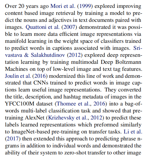
Over 20 years ago Mori et al. (1999) explored improving content based image retrieval by training a model to predict the nouns and adjectives in text documents paired with images.

This is the foundational concept in its simplest form. “Content-based image retrieval” is the task of finding similar images to a query image. Mori et al. realized that the text accompanying an image (like in an article) provides valuable clues. By training a model to associate parts of an image with specific words (nouns and adjectives), they could improve their system. This early work established the core principle: text paired with images is a powerful source of supervision.

The idea continued to evolve with increasing sophistication through the 2000s and early 2010s with work from Quattoni et al. (2007) and Srivastava & Salakhutdinov (2012), who explored more advanced techniques for learning “deep representations” from multimodal (i.e., multiple types of data, like text and images) features.

The Modern Era: CNNs Meet Text

The real acceleration began when modern deep learning architectures, specifically Convolutional Neural Networks (CNNs), were applied to the problem.

Joulin et al. (2016) modernized this line of work and demonstrated that CNNs trained to predict words in image captions learn useful image representations. They converted the title, description, and hashtag metadata of images in the YFCC100M dataset … into a bag-of-words multi-label classification task and showed that pre-training AlexNet … learned representations which preformed similarly to ImageNet-based pre-training on transfer tasks.

This was a major milestone. Joulin et al. took a large dataset of images from Flickr, each with associated text (titles, hashtags, etc.). They treated this as a massive classification problem using a bag-of-words (BoW) approach.

• Bag-of-Words (BoW): This is a simple way to represent text. Imagine you take a sentence, throw all the words into a bag, and shake it up. You ignore grammar and word order, and just count the occurrences of each word. The model’s task was to look at an image and predict the “bag of words” that appeared in its description.

The crucial finding was that an AlexNet model (the CNN that kicked off the deep learning boom in 2012) pre-trained this way learned visual features that were just as useful as those learned from the meticulously-labeled ImageNet dataset. This was strong evidence that learning from messy, real-world text could compete with learning from clean, human-labeled categories.

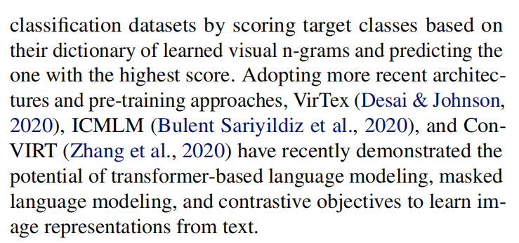
Li et al. (2017) then extended this approach to predicting phrase n-grams in addition to individual words and demonstrated the ability of their system to zero-shot transfer to other image classification datasets…

Li et al. took the next logical step. Instead of just predicting individual words (1-grams), they trained their model to predict n-grams (sequences of n words). For example, instead of predicting “golden” and “retriever” separately, the model could predict the 2-gram “golden retriever.” This captures more meaning. More importantly, they were one of the first to show that this approach could enable zero-shot transfer. They could create a classifier for new, unseen categories just by describing them with text. While the performance was low (as the paper later notes), it was a critical proof of concept.

The Immediate Predecessors

The final pieces of the puzzle came from very recent work that incorporated the latest NLP architectures and training techniques.

Adopting more recent architectures and pre-training approaches, VirTex (Desai & Johnson, 2020), ICMLM (Bulent Sariyildiz et al., 2020), and ConVIRT (Zhang et al., 2020) have recently demonstrated the potential of transformer-based language modeling, masked language modeling, and contrastive objectives to learn image representations from text.

These papers, published just before CLIP, brought the vision-language field right up to the cutting edge. They incorporated ideas from the NLP revolution we discussed earlier, like using powerful Transformer models to understand the text.

Most importantly, they explored contrastive objectives. This is a key concept for understanding CLIP.

• Contrastive Objectives: Instead of a predictive task (e.g., “predict the exact words in this caption”), a contrastive task is a matching task. The model is given an image, one correct text caption, and several incorrect captions. Its only job is to learn which text is the correct match. It learns to pull the representations of the correct (image, text) pair together in its embedding space, while pushing the representations of incorrect pairs far apart. This is often a much more efficient and robust learning signal than trying to predict every single word correctly.

These papers served as the final “proofs of concept,” showing that combining modern architectures with a contrastive learning objective was a promising path forward. The stage was now set for the CLIP authors to ask: what happens if we take this exact approach and scale it up… way up?

The Performance Gap and the “Pragmatic Middle Ground”

If learning from natural language is such a great idea, why wasn’t everyone already doing it? The authors directly address this by pointing to a simple, unavoidable fact: the performance just wasn’t good enough.

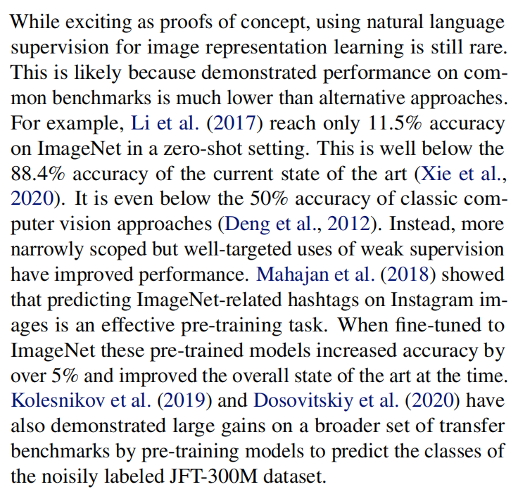
While exciting as proofs of concept, using natural language supervision for image representation learning is still rare. This is likely because demonstrated performance on common benchmarks is much lower than alternative approaches. For example, Li et al. (2017) reach only 11.5% accuracy on ImageNet in a zero-shot setting.

This is the sober reality check. The earlier work by Li et al. was a fantastic proof of concept for zero-shot transfer, but an 11.5% accuracy on ImageNet is, to put it bluntly, terrible. The authors drive this point home by providing two stark comparisons:

1. It was far below the 88.4% accuracy of the state-of-the-art models at the time.
2. It was even worse than the 50% accuracy of “classic” (pre-deep learning) computer vision methods from nearly a decade prior.

With such poor performance, it’s no wonder that this approach remained a niche research area rather than a mainstream technique. The promise of flexibility was overshadowed by the reality of poor results.

However, this didn’t stop researchers from using large-scale, internet-style data. Instead, they found a successful “middle ground” by using a more targeted, albeit less flexible, form of supervision.

Instead, more narrowly scoped but well-targeted uses of weak supervision have improved performance. Mahajan et al. (2018) showed that predicting ImageNet-related hashtags on Instagram images is an effective pre-training task.

This introduces a key concept: weak supervision. This term refers to using labels that are noisy, imprecise, or not perfectly curated, in contrast to the “gold-standard” clean labels of a dataset like ImageNet. The key insight from Mahajan et al. was to leverage this at a massive scale.

• What they did: They trained a model on billions of public Instagram images. The “label” for each image was simply the set of hashtags its user had applied.
• Why it’s “weak”: Hashtags are very noisy. An image of a cat at the beach might be tagged with #cat, #beach, #sunset, and #vacation.
• Why it’s “well-targeted”: Crucially, they filtered the hashtags to only include those relevant to the 1000 ImageNet classes.
• The Result: This was an incredibly effective pre-training strategy. A model pre-trained on these noisy hashtags and then fine-tuned on ImageNet achieved a new state-of-the-art accuracy, boosting performance by over 5%.

This was followed by similar work that further validated the approach:

Kolesnikov et al. (2019) and Dosovitskiy et al. (2020) have also demonstrated large gains on a broader set of transfer benchmarks by pre-training models to predict the classes of the noisily labeled JFT-300M dataset.

This work used JFT-300M, a massive internal Google dataset with 300 million images and noisy, automatically generated labels for thousands of classes. Just like the Instagram work, pre-training on this huge, “weakly” labeled dataset before fine-tuning on smaller, clean datasets led to huge performance gains.

So, the authors have established a clear story:

1. The dream of learning from general, arbitrary text (like captions) was exciting but performed poorly.
2. The pragmatic approach of learning from massive but targeted weak labels (like hashtags or noisy class labels) was a huge success for pre-training.

This sets the stage for the authors to critique this successful “middle ground” and introduce their own approach as the true solution.

The Problem with the Middle Ground: A Critique of Weak Supervision

The successful pre-training methods from Instagram and Google (JFT-300M) represented a huge step forward. The authors acknowledge this, calling it the “pragmatic middle ground.”

This line of work represents the current pragmatic middle ground between learning from a limited amount of supervised “gold-labels” and learning from practically unlimited amounts of raw text.

Think of it as a spectrum of supervision:

• One Extreme: A small set of high-quality, human-verified “gold labels” (e.g., ImageNet).
• The Other Extreme: A nearly infinite amount of messy, unstructured, raw text paired with images (the authors’ ultimate goal).
• The Middle Ground: Massive datasets of “weakly” labeled images (e.g., Instagram hashtags). This approach successfully captured the scale of the internet data but constrained the supervision to be more like traditional labels.

However, the authors argue that this pragmatic solution comes with a major compromise that limits its ultimate potential.

However, it is not without compromises. Both works carefully design, and in the process limit, their supervision to 1000 and 18291 classes respectively. Natural language is able to express, and therefore supervise, a much wider set of visual concepts through its generality.

This is the core of the critique. Even though these models were trained on billions of images, the supervision was still a fixed list of categories. It might be a much bigger list than ImageNet’s 1000 classes, but it is a list nonetheless. This fundamentally restricts what the model can learn. If a concept isn’t in your list of 18,291 target labels, the model has no way to learn it.

Natural language, by contrast, is not a list. It is a general-purpose system for describing the world. It can express an almost infinite variety of visual concepts: objects (“dog”), actions (“a dog jumping”), attributes (“a fluffy brown dog”), relationships (“a dog chasing a cat”), and abstract ideas (“a lonely dog”). This is the expressiveness and generality the authors want to capture.

The second, more technical limitation is baked into the architecture of these “middle ground” models.

Both approaches also use static softmax classifiers to perform prediction and lack a mechanism for dynamic outputs. This severely curtails their flexibility and limits their “zero-shot” capabilities.

This is a crucial technical point. Let’s break it down:

• Static Softmax Classifier: As we discussed in our earlier note, this refers to the final layer of a traditional classification model. It has a fixed number of outputs, one for each class in the predefined list. The softmax function then converts these outputs into a probability distribution over that fixed list.
• Lack of Dynamic Outputs: Because the classifier’s structure is fixed, it cannot produce outputs for new, unseen classes. It is architecturally locked into its original set of categories.

This architectural choice makes true, flexible zero-shot transfer impossible. You cannot simply give the model a new text description at test time and have it classify an image, because there is no output neuron corresponding to that new concept. The model’s knowledge is trapped behind this rigid, static classifier.

In essence, the authors are arguing that while the weak supervision approach was a powerful trick for boosting performance on existing benchmarks, it was an evolutionary dead end. To achieve their goal of a truly flexible, general-purpose vision model, they needed to abandon the fixed-classifier paradigm entirely, a problem that would require a different approach to both the data and the model.

Closing the Gap with Scale: Introducing CLIP

The authors now identify the final, crucial difference between the successful “weak supervision” models and the less successful attempts at learning from general natural language: scale.

A crucial difference between these weakly supervised models and recent explorations of learning image representations directly from natural language is scale. While Mahajan et al. (2018) and Kolesnikov et al. (2019) trained their models for accelerator years on millions to billions of images, VirTex, ICMLM, and ConVIRT trained for accelerator days on one to two hundred thousand images.

This is a critical insight. The successful models weren’t just successful because they used targeted hashtags; they were successful because they were trained on an absolutely colossal scale.

• Weak Supervision Models (Instagram, JFT-300M): Trained on billions of images, requiring accelerator-years of compute. An “accelerator-year” is the equivalent of running a single high-end GPU or TPU for a full year, 24/7.
• Natural Language Supervision Models (VirTex, etc.): Trained on only hundreds of thousands of images, requiring only accelerator-days of compute.

The authors are hypothesizing that the previous attempts at learning from general language failed not because the idea was wrong, but because they were orders of magnitude too small. The rich, noisy, and complex signal of natural language might require a massive amount of data to work effectively.

This leads directly to their own contribution.

In this work, we close this gap and study the behaviors of image classifiers trained with natural language supervision at large scale. Enabled by the large amounts of publicly available data of this form on the internet, we create a new dataset of 400 million (image, text) pairs and demonstrate that a simplified version of ConVIRT trained from scratch, which we call CLIP, for Contrastive Language-Image Pre-training, is an efficient method of learning from natural language supervision.

Here, they lay out the core components of their work:

1. Close the Scale Gap: They are the first to attempt training with general natural language supervision at the same massive scale as the successful weak supervision methods.
2. A New Dataset: To do this, they had to build their own dataset from scratch, collecting 400 million image-text pairs from the internet. This is a monumental engineering effort and a key contribution in itself.
3. The Method (CLIP): They name their model CLIP, which stands for Contrastive Language-Image Pre-training. They explicitly state it’s a simplified version of the ConVIRT model (one of the immediate predecessors they mentioned), which uses the efficient and robust contrastive learning objective we discussed earlier.

Finally, they summarize the key findings they will present in the rest of the paper.

We study the scalability of CLIP by training a series of eight models… and observe that transfer performance is a smoothly predictable function of compute… We find that CLIP, similar to the GPT family, learns to perform a wide set of tasks during pre-training including OCR, geo-localization, action recognition, and many others. We measure this by benchmarking the zero-shot transfer performance of CLIP on over 30 existing datasets…

This is the roadmap for the rest of the paper. They will show that:

• CLIP’s performance scales predictably with model size and compute, just like the GPT models did for NLP. This is a strong sign that the approach is robust and has not yet hit its limits.
• During pre-training, CLIP learns a surprising variety of skills beyond simple object recognition.
• They will prove its capabilities by testing its zero-shot transfer performance on a very broad and diverse set of over 30 benchmarks.

This paragraph perfectly concludes the setup and transitions us into the main body of the paper, where the authors will provide the evidence to back up these claims.

2. Approach

2.1 Natural Language Supervision

At the heart of CLIP is a single, powerful idea that serves as the foundation for all the technical details that follow.

At the core of our approach is the idea of learning perception from supervision contained in natural language.

This is their guiding principle. Instead of learning from predefined class labels like class_id: 7 (which a file might later map to “car”), the model learns directly from the raw text that humans use to describe the world: “a photo of a blue car parked on the street.”

A Tangle of Terminology

The authors first take a moment to clear up some confusion. The field of machine learning has many different terms for training without clean, human-provided labels, and the lines can get blurry.

…terminology used to describe work in this space is varied, even seemingly contradictory… [approaches are described] as unsupervised, self-supervised, weakly supervised, and supervised respectively.

Imagine one paper scrapes image-caption pairs and calls the method “supervised” because the captions are technically labels. Another paper might do the same but call it “weakly supervised” because the captions are noisy. A third might call it “self-supervised” because the labels come from the data itself.

The authors of CLIP argue that these distinctions miss the point. The important, common thread is not the specific implementation, but the source of the training signal. To unify this, they propose their own term: Natural Language Supervision.

We emphasize that what is common across this line of work is not any of the details of the particular methods used but the appreciation of natural language as a training signal. All these approaches are learning from natural language supervision.

This is a key contribution in itself. They are giving a name to the paradigm they are championing, framing it as the defining characteristic of this entire line of research.

Why Natural Language Supervision?

The authors argue that this approach has two game-changing advantages over other methods, from traditional supervised learning to even other forms of self-supervision.

1. It’s Immensely Scalable.

Creating a high-quality, labeled dataset like ImageNet is a monumental undertaking. It requires thousands of hours of human labor to manually classify millions of images, often through a voting process to create a single, canonical “gold label” for each image. This process is slow, expensive, and doesn’t scale easily.

It’s much easier to scale natural language supervision compared to standard crowd-sourced labeling for image classification since it does not require annotations to be in a classic “machine learning compatible format”… Instead, methods which work on natural language can learn passively from the supervision contained in the vast amount of text on the internet.

In contrast, the internet is already filled with billions of images that are naturally paired with text. Scraping this data is an engineering challenge, but it’s a process that can be automated and scaled far more easily than manual labeling.

2. It Enables Flexible Zero-Shot Transfer.

This is the most critical advantage and what truly sets CLIP’s approach apart. Many self-supervised methods are excellent at learning powerful image features. For example, a model might learn to recognize that two different, augmented views of the same cat image should have a similar feature representation.

The problem? That representation is just a vector of numbers. It has no inherent connection to human concepts. After pre-training, you still need a labeled dataset to train a classifier that learns to map those feature vectors to class labels like “cat” or “dog.”

Learning from natural language also has an important advantage over most unsupervised or self-supervised learning approaches in that it doesn’t “just” learn a representation but also connects that representation to language which enables flexible zero-shot transfer.

Natural Language Supervision solves this problem by design. From the very beginning, the model is forced to build a bridge between the visual world and the world of human language. It learns to create image representations that are inherently aligned with the text representations of what those images contain. This built-in connection to language is the key that unlocks CLIP’s remarkable ability to perform classification on tasks and categories it has never seen before.

2.2 Creating a Sufficiently Large Dataset

A model is only as good as the data it’s trained on. For a task as ambitious as learning general visual concepts from language, the CLIP authors needed an engine fueled by an unprecedented amount of diverse, high-quality data. In this section, they explain why existing datasets were not up to the task.

Why Existing Datasets Weren’t Enough

The authors begin by evaluating the common datasets used for this kind of vision-language research. They quickly find them lacking in one of two key areas: scale or quality.

Existing work has mainly used three datasets, MS-COCO (Lin et al., 2014), Visual Genome (Krishna et al., 2017), and YFCC100M (Thomee et al., 2016).

Let’s break down the limitations of each:

• MS-COCO and Visual Genome: These are the gold standard for quality. They contain images with detailed, human-written captions describing the scene. The problem? They are tiny by modern standards, with only about 100,000 training images each. This is simply not enough data to learn the rich, generalizable representations the authors are aiming for, especially when compared to the billion-image datasets used in the “weak supervision” work.

• YFCC100M: This dataset, a collection of 100 million photos from Flickr, seems to solve the scale problem. However, it fails on quality. The “text” associated with these images is often not useful natural language.

Many images use automatically generated filenames like 20160716_113957.JPG as “titles” or contain “descriptions” of camera exposure settings. After filtering to keep only images with natural language titles and/or descriptions in English, the dataset shrunk by a factor of 6 to only 15 million photos. This is approximately the same size as ImageNet.

This is the killer finding. The one public dataset that seemed large enough for the task ended up being no better than ImageNet after basic quality filtering. This neatly demonstrates the core problem: no publicly available dataset had both the massive scale and the natural language supervision required to truly test their hypothesis.

Building a New Dataset: WebImageText (WIT)

Faced with this data gap, the authors made a critical decision: they would build their own.

To address this, we constructed a new dataset of 400 million (image, text) pairs collected form a variety of publicly available sources on the Internet.

This is a monumental contribution. They created a new dataset, which they later call WebImageText (WIT), that is more than 25 times larger than the filtered YFCC100M dataset.

Crucially, they didn’t just scrape images randomly. They designed a systematic process to ensure the dataset covered a vast and diverse range of visual concepts.

To attempt to cover as broad a set of visual concepts as possible, we search for (image, text) pairs as part of the construction process whose text includes one of a set of 500,000 queries.

How did they create this list of 500,000 queries? The footnote reveals a clever and highly effective strategy:

• They started with every word that appears at least 100 times in the English Wikipedia. This provides a massive base of common and uncommon nouns, verbs, adjectives, and proper nouns.
• They augmented this list with bi-grams (two-word phrases) that are statistically significant (i.e., they appear together more often than by chance, like “San Francisco”).
• They also included the titles of all Wikipedia articles above a certain popularity threshold.

This systematic approach ensures their dataset isn’t just large but also incredibly broad, providing the rich and varied supervision needed to learn a truly general model of the visual world. Building this dataset was a foundational step that made the rest of CLIP’s success possible.

2.3 Selecting an Efficient Pre-Training Method

Having established the need for a massive dataset, the authors faced their next great challenge: how do you actually train a model on 400 million images without it taking decades? Training efficiency, they realized, was not just a convenience—it was the key to making their entire approach feasible.

State-of-the-art computer vision systems use very large amounts of compute. Mahajan et al. (2018) required 19 GPU-years to train their ResNeXt101… When considering that both these systems were trained to predict only 1000 ImageNet classes, the task of learning an open set of visual concepts from natural language seems daunting.

The authors start by framing the problem. Previous state-of-the-art models required enormous amounts of computation (e.g., 19 GPU-years) just to learn 1000 fixed categories. Their goal of learning a nearly unlimited set of concepts from noisy, complex natural language was far more ambitious. A slow, inefficient training method would be a non-starter. This led them to a crucial bake-off between three different approaches.

Attempt 1: Predictive Language Modeling (Too Slow)

Their first attempt was the most direct and, in some ways, the most intuitive. It was similar to the approach used by VirTex, one of the recent papers they cited.

Our initial approach, similar to VirTex, jointly trained an image CNN and text transformer from scratch to predict the caption of an image. However, we encountered difficulties efficiently scaling this method.

In this setup, the model would look at an image and then, using a Transformer-based language model, try to generate the exact caption associated with it, word by word.

The problem? This is an incredibly difficult and unforgiving task. The text paired with an image on the internet can vary wildly. A photo of a cat might be paired with “a picture of my cat, Fluffy,” or “a cat sitting on a sofa,” or “here’s a cute animal #catsofinstagram.” Forcing the model to predict the exact sequence of words is a very high bar and, as they found, a very slow way to learn. As shown in their Figure 2, this approach was three times slower at learning to recognize ImageNet classes than a simpler baseline.

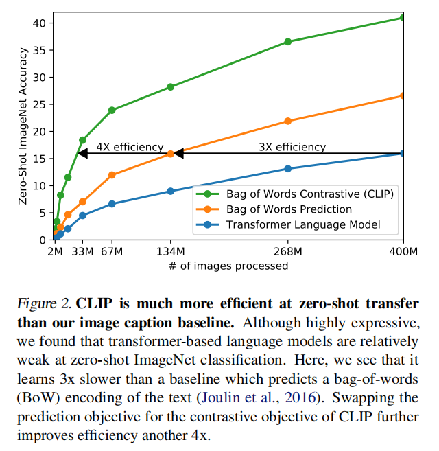
Attempt 2: Bag-of-Words Prediction (Better, But Not Enough)

The simpler baseline they compared against was the bag-of-words (BoW) approach, similar to the one used by Joulin et al. (2016). Instead of predicting the exact sentence, the model’s task was simply to predict the set of words present in the caption, ignoring grammar and word order. This is an easier task and, as expected, it was more efficient than full language modeling. However, it still wasn’t the breakthrough in efficiency they needed.

The Winner: Contrastive Learning (4x More Efficient)

This led them to their third and final approach, which solved the efficiency puzzle by reframing the problem entirely.

…we explored training a system to solve the potentially easier proxy task of predicting only which text as a whole is paired with which image and not the exact words of that text. … Starting with the same bag-of-words encoding baseline, we swapped the predictive objective for a contrastive objective in Figure 2 and observed a further 4x efficiency improvement…

This is the core of CLIP’s training method. Instead of predicting the caption (a generative task), they turned it into a matching task (a contrastive task). Here’s how it works:

1. Take a batch of N images and their N corresponding text captions.
2. This creates N correct pairs. All other combinations (N*N - N of them) are incorrect.
3. The model’s goal is to learn a representation for images and text such that the similarity score for the correct pairs is high, and the similarity score for all incorrect pairs is low.

This is a much more efficient learning signal. The model doesn’t get punished for minor wording differences in a caption; it just has to learn that “a photo of a dog” is a better match for a dog image than “a photo of a cat” is. This simple change provided a massive 4x efficiency boost over the already-better BoW method. Combined with the 3x improvement over the language modeling approach, the contrastive objective was up to 12 times more efficient, making it the clear winner and the right choice for training at scale.

The CLIP Objective: A Simplified and Scalable Contrastive Loss

The paper then provides the technical details of their contrastive approach.

Given a batch of N (image, text) pairs, CLIP is trained to predict which of the N × N possible (image, text) pairings across a batch actually occurred. To do this, CLIP learns a multi-modal embedding space by jointly training an image encoder and text encoder to maximize the cosine similarity of the image and text embeddings of the N real pairs in the batch while minimizing the cosine similarity of the embeddings of the N^2 − N incorrect pairings.

This method, known formally as the InfoNCE loss, was becoming popular in self-supervised learning, and the authors adapted it for their vision-language task. They also made several key simplifications compared to other contemporary methods, demonstrating the robustness of the core idea:

• They trained the model from scratch, without using pre-trained ImageNet weights for the image encoder or a pre-trained language model for the text encoder.
• They used a simple linear projection to map the encoder outputs into the multi-modal embedding space, forgoing the more complex non-linear projection heads used by models like SimCLR.
• They used minimal data augmentation: just a single random square crop from the resized images.
• They even optimized the temperature parameter of the softmax function, a small but important hyperparameter, directly during training.

These simplifications show that the power of CLIP doesn’t come from lots of complex tricks or architectural bells and whistles. It comes from a simple, highly efficient contrastive objective applied to a massive and diverse dataset.

TipA Quick Note: What is a “Projection Head” and Why Did CLIP Use a Simple One?

In the paper, the authors state they used a “simple linear projection” instead of the “more complex non-linear projection heads” used by other models like SimCLR. This might sound like technical jargon, but it’s a key architectural choice that’s worth understanding.

At its core, the issue is about how you get from the raw output of an encoder to the final space where you perform the contrastive learning (the matching game).

The Standard Approach at the Time: The Non-Linear Projection Head

In many self-supervised and contrastive learning frameworks, particularly SimCLR (a very influential paper on contrastive learning for images), the process looked like this:

1. Encoder: An image goes into a powerful encoder (e.g., a ResNet) which produces a feature vector, let’s call it h. This vector h is the rich, general-purpose representation of the image that you want to use for downstream tasks later on.
2. Projection Head: The feature vector h is not used directly for the contrastive loss. Instead, it’s passed through a small neural network, typically a Multi-Layer Perceptron (MLP), called the “projection head.” This MLP transforms h into a new vector, z.
3. Contrastive Loss: The contrastive learning (the matching game of pulling similar things together and pushing different things apart) is performed on these final z vectors.
4. Discard after Training: Crucially, after pre-training is finished, the projection head is thrown away. For any downstream task (like classification), you use the original feature vectors, h, that came directly from the encoder.

Why do this? The theory behind SimCLR’s approach was that this separation was beneficial. The projection head’s job was to transform the features into a space where it’s easy to perform the contrastive task. This process might involve throwing away some information that’s not useful for the matching game (e.g., precise color information might be discarded if the task is just to match two augmented views of the same object).

By adding this extra step, you allow the main encoder’s representation h to remain as rich and general as possible, retaining all that potentially useful information, while the disposable projection head does the “dirty work” of preparing the features for the contrastive loss.

CLIP’s Simpler Approach: The Linear Projection

The CLIP authors decided to simplify this entire process.

1. Encoder: An image (or text) goes into its respective encoder, producing a feature vector.
2. Linear Projection: Instead of a multi-layer MLP, this feature vector is passed through a single, simple linear layer (essentially, just one matrix multiplication). This transforms the vector into the final representation used in the contrastive space.

What does this mean? A linear projection is much less powerful than a non-linear MLP. It can only perform basic transformations like rotating and scaling the feature space; it can’t learn complex, non-linear relationships.

By making this choice, the CLIP authors are making an implicit statement: the representations coming directly out of our encoders are already good enough. They don’t need a powerful, complex transformation to be prepared for the contrastive learning task. The raw features can be mapped directly into the shared multi-modal embedding space with a simple, learned linear map.

Why did they make this choice?

• Simplicity and Efficiency: It’s a simpler architecture with fewer parameters.
• It Just Worked: As the authors state, “We did not notice a difference in training efficiency between the two versions.” This suggests that with their massive dataset and the strong signal from the language-image objective, the extra complexity of the non-linear head was simply unnecessary.
• A Different Problem: They speculate that the non-linear head might be specifically beneficial for image-only self-supervised learning, where the task is to identify two augmented views of the same image. In CLIP’s case, the task is to match a photo with a sentence — a fundamentally different and perhaps clearer signal that doesn’t require the extra transformation.

TipA Quick Note: The “Confidence Knob,” or Why Learnable Temperature is a Clever Trick

In the paper, the authors mention that the “temperature parameter… is directly optimized during training.” This might seem like a minor detail, but it’s a clever and pragmatic solution to a notoriously difficult problem in contrastive learning. To understand why, let’s think of this parameter as the model’s “confidence knob.”

1. What is Softmax Temperature?

First, a quick refresher. In classification, a model often outputs raw scores, called logits. The softmax function then converts these logits into a clean probability distribution (a set of numbers that add up to 1).

The temperature (let’s call it T) is a parameter that controls the shape of this probability distribution. It works by dividing the logits before they are fed into the softmax function:

probabilities = softmax(logits / T)

The effect of T is as follows:

• High Temperature (e.g., T > 1): This makes the probabilities “softer” or more uniform. The model becomes less confident. A high T shrinks the logits, making the differences between them smaller. For example, logits of [10, 0, -10] might become probabilities of [0.6, 0.2, 0.2].
• Low Temperature (e.g., T < 1): This makes the probabilities “sharper” or more “peaked.” The model becomes more confident. A low T exaggerates the differences between the logits. The same logits of [10, 0, -10] might become probabilities of [0.99, 0.01, 0.0].

2. The Goldilocks Problem in Contrastive Learning

In CLIP’s contrastive setup, the “logits” are the similarity scores between an image and all the text captions in a batch. The model’s goal is to assign a very high probability to the one correct match. The temperature here is crucial for controlling the learning process:

• If T is too high (too soft): The model will be unconfident. The probability of the correct pair will only be slightly higher than the incorrect pairs. This creates a very weak learning signal (a small gradient), and the model will learn very slowly or not at all.
• If T is too low (too sharp): The model will be overconfident. It might quickly learn to separate the “easy” negative examples (e.g., a dog image vs. the caption “a photo of a car”) but fail to learn from the “hard” negative examples (e.g., a dog image vs. the caption “a photo of a wolf”). This can lead to poor training and a worse final model.

You need a temperature that is “just right”—a value that properly balances the penalties for incorrect pairings and creates a stable, effective learning signal.

3. The Old Way: Expensive and Painful Hyperparameter Tuning

Traditionally, the temperature T is a hyperparameter. This means it’s a value that the data scientist has to choose and set before training begins. How do you find the best value?

The standard method is a brute-force approach like a grid search. You would run a series of small-scale experiments, trying a fixed T of 0.01, then 0.05, then 0.07, then 0.1, and so on. You’d then pick the value that worked best and use it for your final, large-scale training run.

For a model like CLIP, which is trained on 400 million images and takes weeks on hundreds of GPUs, this process is prohibitively expensive. Running multiple experiments just to tune one knob is not a feasible option.

4. CLIP’s Elegant Solution: Let the Model Learn the Knob’s Setting

Instead of manually guessing the best temperature, the CLIP authors did something much smarter: they made the temperature a learnable parameter.

Just like the millions of other weights in the neural network, the temperature T was initialized at some value and then updated at every step of training via backpropagation and gradient descent. The model itself was tasked with figuring out the optimal “confidence level” that best helped it minimize the overall loss. If the model was too unconfident, the loss function would effectively “tell” it to lower the temperature. If it was too overconfident, it would tell it to raise it.

This is more than just a minor tweak; it’s a perfect example of CLIP’s design philosophy:

• It automates a difficult process: It removes the need for the human researcher to perform an expensive and time-consuming hyperparameter search.
• It’s more efficient: It saves a massive amount of computation that would have been wasted on tuning experiments.
• It’s potentially more robust: The model can find a more optimal value for T than a human might through a coarse grid search.

By making the temperature learnable, the authors simplified their training pipeline and made their entire large-scale experiment more practical and likely to succeed.

2.4 Choosing and Scaling a Model

With the dataset and training objective settled, the final piece of the puzzle was the model architecture itself. What kind of neural networks should be used for the image and text encoders, and more importantly, how can they be scaled up effectively to handle the massive dataset?

The Image Encoder: The Workhorse vs. The New Challenger

The authors evaluated two different families of architectures for the image encoder, representing both the established state-of-the-art and a new, promising alternative.

1. The Workhorse: A Modernized ResNet

The first choice was a ResNet-50. The Residual Network (ResNet) architecture is one of the most influential and widely used in computer vision history. It’s a known, reliable “workhorse.” However, the authors didn’t just use the original 2016 version. They made several key modernizations to boost its performance:

• They incorporated ResNet-D improvements, a series of small but effective tweaks to the internal structure of the ResNet blocks.
• They added antialiased blur pooling, a technique that helps the model be less sensitive to small shifts or translations in an image, improving its overall robustness.
• Most interestingly, they replaced the standard “global average pooling” layer with an attention pooling mechanism. Instead of just taking a simple average of all the features at the end of the network, this new layer uses a Transformer-style multi-head attention mechanism to learn a weighted average. In essence, it learns to pay more attention to the most important parts of the image when creating its final summary representation.

2. The New Challenger: The Vision Transformer (ViT) The second architecture they tested was the Vision Transformer (ViT), which was a very new and exciting development at the time. The ViT radically rethinks image processing by applying the Transformer architecture, which was originally designed for text, directly to images. It works by:

• Breaking an image down into a grid of small, fixed-size patches (e.g., 16x16 pixels).
• Treating this sequence of patches as if it were a sequence of words in a sentence.
• Feeding this sequence into a standard Transformer encoder to learn the relationships between the different parts of the image.

The authors followed the original ViT implementation closely, making only a minor modification. By testing both ResNets and ViTs, they were able to compare a mature, highly-optimized CNN against a powerful new paradigm.

The Text Encoder: A Standard Transformer

The choice of text encoder was more straightforward. They used a standard Transformer architecture, very similar to the one used in models like GPT-2. The key details are:

• Architecture: A 12-layer, 512-unit-wide Transformer with 8 attention heads.
• Tokenization: The text is processed using a byte-pair encoding (BPE) tokenizer with a vocabulary of about 49,000 “tokens.” BPE is a clever way to handle language: instead of just splitting words, it breaks words down into common sub-word units. This allows it to represent any word, even ones it has never seen before, without having an enormous vocabulary.
• Processing: For any given text input, the sequence of tokens is capped at 76, bracketed with [SOS] (start of sentence) and [EOS] (end of sentence) tokens. The final representation of the [EOS] token is taken as the feature representation for the entire text snippet, as this token’s final state is influenced by all the words that came before it.

The Scaling Strategy: Growing Smarter, Not Just Bigger

How do you make a model more powerful? The naive approach is to just make it deeper (add more layers) or wider (add more units per layer). However, work from the EfficientNet paper (Tan & Le, 2019) showed that the best strategy is compound scaling: simultaneously increasing the model’s depth, width, and the resolution of the input images in a balanced way.

The CLIP authors adapted this sophisticated strategy for their ResNet models. Instead of painstakingly tuning the exact ratio for each dimension, they used a simple rule of thumb: they allocated additional compute equally to increasing the width, depth, and resolution. This allowed them to create a series of progressively larger and more powerful ResNet models in a principled way.

Interestingly, for the text encoder, they found that performance was much less sensitive to its size. As a result, when scaling up their models, they only scaled the width of the text Transformer, keeping its depth (number of layers) constant. This is a great example of the empirical, results-driven engineering required to build such a massive system.

TipA Quick Note: What is ResNet-D and Why Does it Matter?

When the CLIP authors chose ResNet as one of their image encoders, they didn’t use the original 2016 version off the shelf. Instead, they incorporated a set of important upgrades from a 2018 paper titled “Bag of Tricks for Image Classification with Convolutional Neural Networks.” One of the key improvements from that paper is a modified architecture known as ResNet-D.

To understand ResNet-D, we first need to understand a subtle flaw in the original ResNet design.

The Flaw in the Original ResNet

A standard ResNet is built from “residual blocks.” These blocks have two paths for information to flow:

1. The Main Path: The input goes through a series of convolutional layers.
2. The Skip Connection (or Shortcut): The original input “skips” over these layers and is added back in at the end.

In some of these blocks, the convolutional path needs to downsample the image (i.e., reduce its spatial resolution, like from 56x56 to 28x28). The original ResNet did this using a stride of 2 in the very first 1x1 convolution of the main path.

The problem? A 1x1 convolution with a stride of 2 effectively throws away 3/4 of the information in the feature map. It only looks at every other pixel, discarding the rest. While this works, it’s an aggressive and inefficient way to downsample, causing a significant loss of information early in the block.

The ResNet-D Improvement

ResNet-D fixes this by making a simple but clever change to the downsampling blocks:

• It moves the stride of 2 from the initial 1x1 convolution to the 3x3 convolution later in the path.

This small change has a big impact. Now, the 3x3 convolution sees all of the input features (it has a stride of 1), and it performs the downsampling itself. Because a 3x3 convolution looks at a larger area (a 3x3 patch of pixels), it can learn a much more effective and information-preserving way to downsample the feature map, rather than just naively discarding 75% of the data.

This is a perfect example of a “trick” that costs almost nothing in terms of computation but leads to a noticeable improvement in model accuracy by preserving more information as it flows through the network. By incorporating ResNet-D, the CLIP authors ensured their CNN baseline was as strong and modern as possible.

TipA Quick Note: What is Blur Pooling and Why is it Important for Robustness?

Another key modernization the authors added to their ResNet was antialiased blur pooling. This technique addresses a fundamental problem with how traditional Convolutional Neural Networks (CNNs) handle small shifts in an image.

The Problem: CNNs are Surprisingly Brittle to Shifts

We often think of CNNs as being “translation invariant,” meaning that if you shift an object slightly in an image, the model’s prediction shouldn’t change. In practice, this isn’t entirely true. A standard CNN can be surprisingly sensitive to small, one-pixel shifts.

The culprit is often the max pooling layer (or a convolution with a stride greater than 1), which is used to downsample the feature maps. Imagine a max pooling layer that looks at a 2x2 grid of pixels and outputs the maximum value. If a key feature is right on the edge of that 2x2 grid, a tiny shift in the input image can cause it to fall into a different grid, leading to a completely different output. This can make the network’s internal representations unstable and brittle.

This violates a core principle of signal processing known as Nyquist’s sampling theorem. In simple terms, if you sample a signal (like an image) too aggressively without smoothing it first, you can get aliasing artifacts—unwanted patterns that distort the true signal. This is exactly what a standard max pooling or strided convolution does.

The Solution: Blur First, Then Sample

Antialiased blur pooling (from the 2019 paper “Making Convolutional Networks Shift-Invariant Again”) solves this problem with an incredibly simple and elegant idea inspired by classic signal processing:

1. Blur: Before downsampling, apply a small, fixed blurring filter (like a 3x3 triangular filter) to the feature map. This has the effect of smoothing it out.
2. Downsample: Now, perform the standard downsampling operation (like max pooling or a strided convolution) on this new, blurred feature map.

By blurring first, you are effectively “spreading out” the features. This makes the downsampling operation much more stable. A small shift in the input will no longer cause a drastic change in the output, because the blurred feature has influence over a slightly larger area.

2.5. Training

With the architecture and scaling strategy defined, the authors now turn to the specifics of the training process. This section highlights the different model configurations they trained and the immense computational resources required.

The Model Zoo: A Fleet of ResNets and ViTs

The authors didn’t just train one final CLIP model. To study how performance scales with compute, they trained a whole family of models of varying sizes. This is crucial for their scientific claim that the benefits of their approach are a predictable function of scale.

They trained a total of eight primary models:

• Five ResNet-based models:
  • A standard ResNet-50 and ResNet-101.
  • Three much larger, custom ResNets built using their EfficientNet-style compound scaling strategy. These are denoted RN50x4, RN50x16, and RN50x64, representing models that use approximately 4x, 16x, and 64x the compute of the base ResNet-50, respectively.
• Three Vision Transformer (ViT) based models:
  • ViT-B/32 (the “Base” ViT model using 32x32 pixel patches).
  • ViT-B/16 (the “Base” ViT model using smaller 16x16 patches, which is more powerful).
  • ViT-L/14 (the “Large” ViT model using 14x14 patches).

All models were trained for a fixed 32 epochs, meaning they saw the entire 400 million image dataset 32 times.

The Training Recipe: Optimization and Hyperparameters

The training setup used a standard but highly optimized recipe for large-scale deep learning:

• Optimizer: They used the Adam optimizer, a very popular and effective choice, with a specific modification called “decoupled weight decay regularization,” which can improve generalization.
• Learning Rate Schedule: The learning rate, which controls how big of a step the optimizer takes at each iteration, was decayed over the course of training using a cosine schedule. This means the learning rate starts high, gradually and smoothly decreases in a cosine curve, and ends near zero. This is a very common and robust schedule for training large models.
• Hyperparameter Tuning: Interestingly, they note that the initial hyperparameters were found by experimenting on the baseline ResNet-50 model. For the larger, more expensive models, these settings were then “adapted heuristically” due to the massive computational cost of doing a full hyperparameter search for each one. This is a pragmatic admission of the real-world constraints of training at this scale.
• Batch Size: They used an absolutely enormous minibatch size of 32,768. This is one of the keys to training large models efficiently on parallel hardware like GPUs and TPUs. A large batch size ensures that the hardware is fully utilized and that the estimate of the gradient at each step is very stable.

The Engineering of Scale: Making it all Fit

Training a model of this magnitude on a dataset this large requires a suite of advanced engineering techniques to manage memory and speed up computation. The authors used several key methods:

• Mixed-Precision Training: Instead of representing all numbers in the network with 32-bit floating point precision (FP32), this technique uses a mix of lower-precision 16-bit floats (FP16) and FP32. FP16 requires half the memory and is often much faster on modern GPUs. This is a standard and essential trick for large-scale training.
• Gradient Checkpointing: A memory-saving technique where, instead of storing all the intermediate activations needed for backpropagation, the model re-computes them on the fly. This trades extra compute for a significant reduction in memory usage, allowing larger models to be trained.
• Sharded Computation: They note that the calculation of the N x N similarity matrix was “sharded,” meaning it was split up across the individual GPUs. Each GPU only had to compute the similarities between its local batch of images and all the text embeddings, rather than having one GPU compute the entire massive matrix.

Finally, the authors provide a sense of the staggering compute involved:

• The largest ResNet model (RN50x64) took 18 days to train on 592 V100 GPUs.
• The largest Vision Transformer model (ViT-L/14) took 12 days on 256 V100 GPUs.

This section makes it clear that CLIP is not just a scientific breakthrough, but also a monumental feat of engineering.

3. Experiments

3.1 Zero-Shot Transfer

The entire premise of CLIP is that its novel pre-training strategy enables flexible transfer to new tasks. In this section, the authors put that claim to the test. But before they show us the results, they take a moment to define exactly what they mean by “zero-shot transfer” and why their definition represents a more ambitious and meaningful measure of a model’s capabilities.

3.1.1 Motivation: Redefining “Zero-Shot” as True Task Learning

The term “zero-shot learning” can mean different things to different people. The authors begin by clarifying the distinction between the traditional, narrow definition and their own broader, more challenging one.

In computer vision, zero-shot learning usually refers to the study of generalizing to unseen object categories in image classification (Lampert et al., 2009). We instead use the term in a broader sense and study generalization to unseen datasets.

The classic definition of zero-shot learning in computer vision often involves a specific setup: a model is trained on a set of seen classes (e.g., horses, dogs) and a list of their semantic attributes (e.g., has_fur, has_hooves, has_tail). At test time, it’s given the attributes for an unseen class (e.g., has_stripes, has_hooves) and must identify a “zebra” from a list of unseen class names, even though it has never seen a zebra image. This tests generalization to a new category within a single, constrained task.

The CLIP authors propose a much harder test: generalization to entirely new datasets. This is a proxy for evaluating a model’s ability to perform new tasks. This reframing is the core of their evaluation philosophy.

While much research in the field of unsupervised learning focuses on the representation learning capabilities of machine learning systems, we motivate studying zero-shot transfer as a way of measuring the task-learning capabilities of machine learning systems.

This is a critical distinction. Let’s break it down:

• Representation Learning: The goal is to learn a good set of features from an image. The standard evaluation is a “linear probe,” where you freeze the features from the pre-trained model and train a simple linear classifier on top of them for a new task. This tests whether the features are good, but not whether the model itself can perform the task.
• Task Learning: The goal is to see if the model can perform a new task directly, with no additional training. For CLIP, this means giving it an image and a set of new text descriptions and seeing if it can make the correct classification. This is a much higher bar. It tests the model’s ability to apply its knowledge in a flexible, zero-shot way. This evaluation philosophy is directly inspired by the work on GPT-2 and GPT-3, which were also benchmarked on their surprising ability to perform tasks they weren’t explicitly trained for.

To illustrate this point further, they draw a clever contrast between two well-known datasets.

While it is reasonable to say that the SVHN dataset measures the task of street number transcription on the distribution of Google Street View photos, it is unclear what “real” task the CIFAR-10 dataset measures.

This is a subtle but powerful argument.

• SVHN (Street View House Numbers): This dataset has a clear, real-world task: reading digits from photos of houses. Testing a model on SVHN zero-shot is a true test of its ability to generalize to the task of number recognition.
• CIFAR-10: This is a classic academic benchmark of low-resolution images. It doesn’t correspond to a specific real-world application. Therefore, testing zero-shot on CIFAR-10 is less a test of “task generalization” and more a test of domain generalization or robustness to distribution shift. Can the model recognize a tiny, blurry car when it was pre-trained on high-resolution internet photos?

This shows the nuance in their approach. By evaluating across more than 30 datasets, they can test not just one capability, but a whole spectrum of generalization skills, from task learning to robustness.

3.1.2 Using CLIP for Zero-Shot Transfer

The real power of CLIP’s pre-training is that the mechanism for zero-shot classification is not a clever hack or an afterthought—it is a direct application of the very task the model was trained to perform.

CLIP is pre-trained to predict if an image and a text snippet are paired together in its dataset. To perform zero-shot classification, we reuse this capability.

The process is straightforward and powerful, turning any set of class names into a dynamic, on-the-fly classifier.

For each dataset, we use the names of all the classes in the dataset as the set of potential text pairings and predict the most probable (image, text) pair according to CLIP.

Let’s walk through the step-by-step process they describe, which we also detailed in our earlier note:

1. Get the Image Embedding: First, an input image is passed through CLIP’s trained image encoder. This produces a single feature vector that represents the visual content of the image.
2. Get the Text Embeddings: Next, you take the list of all possible class names for the dataset you want to test on (e.g., for CIFAR-10, this would be “plane”, “car”, “bird”, “cat”, etc.). Each of these class names is passed through CLIP’s trained text encoder. This produces a set of feature vectors, one for each class name.
3. Calculate Similarity: The cosine similarity is then calculated between the single image embedding and each of the text embeddings. This results in a list of scores (logits), one for each class, representing how “close” the image is to the concept described by each text label.
4. Normalize to Probabilities: These similarity scores are then scaled by the learned temperature parameter and converted into a probability distribution using a softmax function. The class with the highest probability is the model’s final prediction.

A New Perspective: The Text Encoder as a “Hypernetwork”

The authors then offer a fascinating reinterpretation of what’s happening under the hood. They frame the whole system not just as two encoders, but as a computer vision backbone paired with a network that generates the weights of a classifier on demand.

When interpreted this way, the image encoder is the computer vision backbone which computes a feature representation for the image and the text encoder is a hypernetwork (Ha et al., 2016) which generates the weights of a linear classifier based on the text specifying the visual concepts that the classes represent.

This is a powerful analogy. Let’s break it down:

• A linear classifier is just a set of weights. For a given image feature vector, you take the dot product of the features with the weights for each class to get the scores.
• A hypernetwork is a neural network that outputs the weights of another neural network.

In CLIP’s zero-shot setup, the text encoder is acting as a hypernetwork. You give it a text description like “a photo of a dog,” and it outputs a vector. This vector is, functionally, the weight vector for the “dog” class in a dynamically generated linear classifier. The cosine similarity calculation is mathematically equivalent to taking the dot product between L2-normalized feature and weight vectors.

This idea of generating a classifier from natural language dates back several years, but CLIP is the first model to make it truly effective at a large scale.

This perspective also provides a novel way to think about the pre-training process itself:

…every step of CLIP pre-training can be viewed as optimizing the performance of a randomly created proxy to a computer vision dataset which contains 1 example per class and has 32,768 total classes defined via natural language descriptions.

This is a beautiful insight. Every single training step, with its massive batch size of 32,768, is like a mini, one-shot classification task. For that single step, the model is trying to correctly classify 32,768 images into 32,768 unique “classes” defined by their captions. By doing this billions of times with different random “datasets,” the model learns a truly general ability to connect any image to any text description.

TipA Quick Note: Understanding CLIP’s Evaluation Philosophy

Before diving into pages of results and tables, the authors of CLIP take a moment to establish how and why they evaluate their model the way they do. This philosophy is just as important as the results themselves and is centered on a more ambitious definition of what a “general purpose” vision model should be able to do.

From “Representation Learning” to “Task Learning”

For years, the standard way to evaluate a pre-trained vision model was to test its representation learning capabilities. The process, often called “linear probing,” works like this:

1. Pre-train a large model on a dataset like ImageNet.
2. Take this model and freeze the weights of all its layers except the very last one.
3. For a new, downstream dataset (e.g., classifying flower species), train a new, simple linear classifier “head” on top of these frozen features.

If the model performs well, it means the pre-training process produced a good, general-purpose set of features. However, this doesn’t test the model’s intrinsic ability to perform the new task; it only tests if its features are useful for someone else (the new classifier) to perform the task.

CLIP’s authors argue for a higher standard: task learning. Inspired by the remarkable capabilities of models like GPT-3, they want to measure if the model can perform a new task directly, with zero additional training. This is the essence of their focus on zero-shot transfer. Instead of asking, “Are the features good?”, they ask, “Can the model itself do the job?”

A Broader Definition of “Zero-Shot”

This new philosophy requires a broader definition of “zero-shot.”

• The Classic Definition: Generalizing to unseen categories within a single, familiar task (e.g., classifying a zebra after only being trained on horses and their attributes).
• CLIP’s Definition: Generalizing to unseen datasets which are a proxy for entirely new tasks. For example, can a model pre-trained on a vast collection of internet images and text instantly perform well on a specialized task like recognizing traffic signs, transcribing street numbers, or classifying satellite imagery?

This is a much more challenging and meaningful benchmark. It tests a model’s flexibility and its ability to apply its learned knowledge to novel problems, which is a key step towards more general AI.

How It Works: A Classifier Generated from Language

The mechanism for this powerful zero-shot transfer is a direct and elegant consequence of CLIP’s pre-training:

1. CLIP is trained to find the best match between a given image and a set of text descriptions. It learns to create a shared “concept space” where an image of a cat and the sentence “a photo of a cat” are mathematically close.
2. To perform zero-shot classification, you simply reuse this capability.
3. You take an image and a list of text labels for your new task (e.g., “a photo of a car,” “a photo of a truck”).
4. You encode both the image and all the text labels into the shared concept space.
5. You then calculate which text description is “closest” to the image. That becomes your prediction.

In this framework, the “classifier” is not a fixed part of the model’s architecture. It is created dynamically, on-the-fly, from whatever list of text descriptions you provide. In a sense, CLIP’s text encoder acts as a “hypernetwork”—a network that generates the weights of a classifier just from being told the names of the classes. This is the simple yet profound idea that enables CLIP’s incredible flexibility.

3.1.3 Initial Comparison to Visual N-Grams

Now for the moment of truth. After all the theory and motivation, how does CLIP’s zero-shot performance actually stack up against the previous state-of-the-art? The authors chose Visual N-Grams (Li et al., 2017) as their primary point of comparison. As we discussed, this was the most relevant predecessor that had also demonstrated zero-shot transfer by learning from image-text pairs from the web.

The results, presented in Table 1 of the paper, are not just an incremental improvement; they represent a seismic leap in capability.

In Table 1 we compare Visual N-Grams to CLIP. The best CLIP model improves accuracy on ImageNet from a proof of concept 11.5% to 76.2% and matches the performance of the original ResNet-50 despite using none of the 1.28 million crowd-labeled training examples available for this dataset.

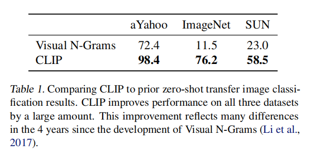
This is the headline result of the entire paper, and it’s worth pausing to fully appreciate its significance.

• The Leap in Accuracy: On the standard ImageNet benchmark, CLIP achieves 76.2% accuracy in a zero-shot setting. This is a nearly 7x improvement over the 11.5% achieved by Visual N-Grams. It elevates the approach from a “proof of concept” to a genuinely useful and powerful method.
• Matching a Fully Supervised Model, with Zero Data: This is the most shocking part. The 76.2% accuracy score matches the performance of the original ResNet-50 model. But the ResNet-50 was explicitly trained on all 1.28 million labeled ImageNet training images. CLIP achieved the same performance without being trained on a single one of them. It did so just by matching the images to text descriptions of the 1000 ImageNet classes. This is a powerful demonstration that learning from vast, noisy natural language on the internet can be as effective as learning from a massive, clean, human-labeled dataset.

The authors also note another impressive result:

Additionally, the top-5 accuracy of CLIP models are noticeably higher than their top-1, and this model has a 95% top-5 accuracy, matching Inception-V4 (Szegedy et al., 2016).

• Top-5 Accuracy: This metric means that the correct label was in the model’s top five predictions 95% of the time. This incredibly high score suggests that even when CLIP’s top guess is wrong, the correct answer is usually very close. This indicates a deep and robust semantic understanding of the visual concepts, on par with another very strong, fully supervised model (Inception-V4).

An Important Caveat: This Isn’t an Apples-to-Apples Fight

The authors, practicing good scientific diligence, are quick to point out that this comparison is not entirely fair.

…the comparison to Visual N-Grams is meant for contextualizing the performance of CLIP and should not be interpreted as a direct methods comparison… many performance relevant differences between the two systems were not controlled for.

The goal here is to show a generational leap, not to claim a direct victory on a level playing field. The key differences were:

• Dataset Size: CLIP was trained on a dataset 10x larger.
• Model and Training Scale: CLIP uses a much larger vision model and likely over 1000x more total training compute.
• Architecture: CLIP uses a modern Transformer-based text encoder, which did not exist when Visual N-Grams was published in 2017.

A Fairer Comparison: The CLIP Objective Still Wins

To address this, the authors ran a more controlled experiment to isolate the benefit of their training method (contrastive learning) from the benefit of their massive new dataset.

As a closer comparison, we trained a CLIP ResNet-50 on the same YFCC100M dataset that Visual N-Grams was trained on and found it matched their reported ImageNet performance within a V100 GPU day.

This is a crucial control experiment. By training their own model on the same dataset as the previous work, they show that the contrastive objective used by CLIP is a far more efficient and effective learning method than the predictive, n-gram-based objective used by Visual N-Grams.

Finally, they note that CLIP’s dominance holds on the other datasets reported by Visual N-Grams as well, achieving a 95% reduction in error on one and more than doubling the accuracy on another. With this initial, powerful result established, they signal their intent to move beyond this small comparison and stress-test CLIP against a much broader suite of over 30 computer vision datasets.

3.1.4 Prompt Engineering and Ensembling: Getting the Best Out of CLIP

For a model that understands vision through the lens of language, the way you talk to it matters immensely. The authors discovered that the raw class names provided by most datasets are a poor way to communicate with CLIP, and they developed two powerful techniques — prompt engineering and ensembling — to dramatically improve its zero-shot performance.

The Problem: The “Raw Label” Distribution Gap

The authors first identify a fundamental mismatch between CLIP’s training data and the data in standard evaluation benchmarks.

It’s relatively rare in our pre-training dataset for the text paired with the image to be just a single word. Usually the text is a full sentence describing the image in some way.

CLIP was trained on rich, descriptive sentences. However, most classification datasets just provide a single word for a label, like cat, dog, or car. This creates a distribution gap. It’s like training someone to understand entire news articles and then testing them by only giving them single, isolated headline words. This lack of context can lead to ambiguity and poor performance.

The First Solution: Prompt Engineering

To bridge this gap, the authors developed a simple but highly effective technique that has come to be known as prompt engineering. Instead of just feeding the model the raw, single-word label, they wrap it in a descriptive sentence, or a “prompt template.”

To help bridge this distribution gap, we found that using the prompt template “A photo of a {label}.” to be a good default that helps specify the text is about the content of the image. This often improves performance over the baseline of using only the label text. For instance, just using this prompt improves accuracy on ImageNet by 1.3%.

This is a remarkably simple fix with a significant impact. By changing the input from just dog to "A photo of a dog.", they provide the text encoder with the kind of sentence-level context it is used to seeing. This seemingly minor change instantly boosted ImageNet accuracy by 1.3%.

This technique is particularly useful for solving the problem of polysemy, where a single word can have multiple meanings.

A common issue is polysemy. When the name of a class is the only information provided to CLIP’s text encoder it is unable to differentiate which word sense is meant due to the lack of context. … This happens in ImageNet which contains both construction cranes and cranes that fly. Another example is found in classes of the Oxford-IIIT Pet dataset where the word boxer is, from context, clearly referring to a breed of dog, but to a text encoder lacking context could just as likely refer to a type of athlete.

By engineering the prompt, you can provide the necessary context to disambiguate the meaning. For the Oxford Pets dataset, using a prompt like "A photo of a {label}, a type of pet." makes it perfectly clear to the model that it should be looking for a Boxer dog, not a human boxer. The authors show that customizing prompts to the specific context of a dataset (e.g., "a satellite photo of a {label}" for satellite imagery) can significantly improve performance.

The Second Solution: Ensembling

The authors took this idea a step further. If one good prompt helps, do multiple different prompts help even more? The answer is a resounding yes. This led to their second technique: ensembling.

We also experimented with ensembling over multiple zero-shot classifiers as another way of improving performance. These classifiers are computed by using different context prompts such as ’A photo of a big {label}” and “A photo of a small {label}”.

Instead of relying on a single prompt template, they generate embeddings for dozens of different ones. For example: "a photo of a {label}", "a cropped photo of a {label}", "a drawing of a {label}", "a photo of a big {label}", etc.

Crucially, they perform the ensembling in an extremely efficient way. Instead of getting the final prediction for each prompt and averaging the probabilities, they average the text embeddings themselves. This creates a single, robust text embedding for each class that represents a blended “average” of many different descriptions. This is computationally “free” at inference time, because the averaged embeddings can be pre-computed and cached. For ImageNet, they used an ensemble of 80 different prompt templates, which improved accuracy by an additional 3.5% over the single default prompt.

The Combined Impact: A “Free” Performance Boost

When combined, these two techniques provide a massive boost to CLIP’s zero-shot performance. On ImageNet, they improved accuracy by nearly 5 percentage points (1.3% from the initial prompt + 3.5% from ensembling).

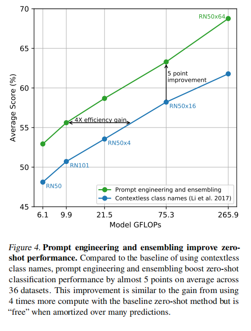
Figure 4 in the paper visualizes this beautifully. The authors plot model performance against the amount of compute (GFLOPs). As models get bigger, performance smoothly increases. But prompt engineering and ensembling provide a large, immediate vertical jump in performance without any increase in model size or compute. This 5-point gain is roughly equivalent to the performance jump you’d get from scaling a model to be four times larger. It’s one of the closest things to a “free lunch” in machine learning: a significant boost in accuracy for almost no additional inference cost.

3.1.5 Analysis of Zero-Shot CLIP Performance

With the core zero-shot mechanism established, the authors conduct a deep dive to contextualize its performance. Is it actually good? Where does it work best? And how does it compare to other learning paradigms like few-shot learning?

How Good is Zero-Shot CLIP? A New Supervised Baseline

Saying CLIP matches the original ResNet-50 is a great headline, but the field has advanced significantly since 2016. To provide a more modern and challenging baseline, the authors compare zero-shot CLIP to a simple but very strong supervised approach.

To contextualize this, we compare to the performance of a simple off-the-shelf baseline: fitting a fully supervised, regularized, logistic regression classifier on the features of the canonical ResNet-50.

Let’s break down this baseline:

• Canonical ResNet-50: The standard, pre-trained ResNet-50 model that is the workhorse of computer vision.
• Features: They take the image representations produced by this ResNet-50 (before its final classification layer).
• Fully Supervised Logistic Regression: They then train a simple linear classifier on top of these features using the entire training set for each of the 27 benchmark datasets.

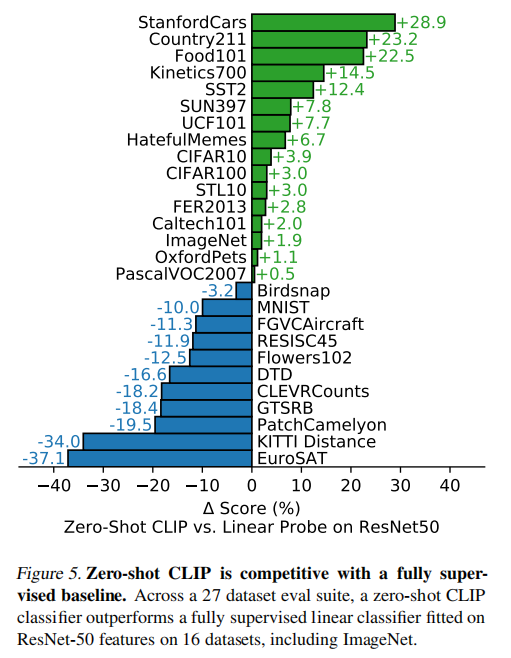
This is a very fair and common way to evaluate the quality of pre-trained features. The results of this comparison, shown in Figure 5, are remarkable. Zero-shot CLIP, without seeing a single training example for any of these 27 tasks, beats the fully supervised ResNet-50 baseline on 16 of the datasets. This is a powerful statement: for a majority of these tasks, a zero-shot instruction to CLIP is more effective than fully training a classifier on thousands of labeled examples from a state-of-the-art ResNet model.

Where Does Zero-Shot CLIP Excel and Where Does It Stumble?

The breakdown of performance across these 27 datasets reveals a clear pattern of strengths and weaknesses.

CLIP’s Strengths:

• Action Recognition: CLIP shows a significant advantage on datasets like Kinetics700 and UCF101. The authors speculate this is because its pre-training on natural language provides a much wider source of supervision for verbs (actions), whereas ImageNet is heavily biased towards nouns (objects).
• General Object Recognition: On classic datasets like ImageNet, CIFAR-10/100, and PascalVOC2007, CLIP’s zero-shot performance is very competitive with the supervised baseline.
• Some Fine-Grained Tasks: It performs exceptionally well on Stanford Cars and Food101, outperforming the baseline by over 20%.

CLIP’s Weaknesses:

Zero-shot CLIP struggles significantly on several types of highly specialized or abstract tasks.

we see that zero-shot CLIP is quite weak on several specialized, complex, or abstract tasks such as satellite image classification (EuroSAT), lymph node tumor detection (PatchCamelyon), counting objects in synthetic scenes (CLEVRCounts), [and] self-driving related tasks…

These failures highlight the limits of the pre-training data. Tasks that require very specific domain knowledge not commonly found in general web text (e.g., medical imaging), or tasks that are more abstract than simple object recognition (e.g., counting), are a major challenge. As the authors wisely caution, for some of these difficult tasks, it may not even be fair to expect a model to succeed with zero prior experience.

Zero-Shot vs. Few-Shot: An Unexpected Result

The most mind-bending comparison in this section is between zero-shot CLIP and few-shot linear classifiers. Intuitively, a one-shot model (which sees one example of each class) should always beat a zero-shot model (which sees none). The authors find that this is surprisingly not the case.

While it is intuitive to expect zero-shot to underperform one-shot, we instead find that zero-shot CLIP matches the performance of 4-shot logistic regression on the same feature space.

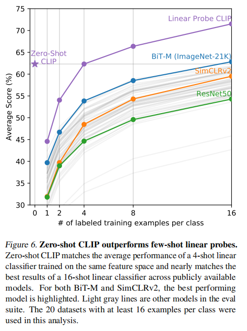
This result, visualized in Figure 6, is astounding. A single text instruction to CLIP is as powerful as showing a standard linear classifier four labeled examples from each class. The authors offer a brilliant explanation for this phenomenon:

1. Zero-Shot is “Communicated”: With a text prompt, you are directly communicating the visual concept you want the model to find. It’s an unambiguous instruction.
2. Few-Shot is “Inferred”: With a handful of examples, the model must infer the target concept. A single image of a dog also contains grass, a sky, a collar, and fur. With only a few examples, it’s very difficult for the model to know which of the many possible visual concepts in the image is the one it’s supposed to learn.

This suggests that for a powerful model like CLIP, a well-crafted text prompt can be a much richer and more efficient learning signal than a small number of ambiguous image examples.

The Final Frontier: How Much Room is Left to Improve?

Finally, the authors ask: how good could zero-shot performance possibly get? To estimate this, they compare zero-shot CLIP’s performance to that of a fully supervised linear classifier trained on CLIP’s own features. This supervised classifier represents a rough upper bound on the performance that is “linearly” extractable from the features.

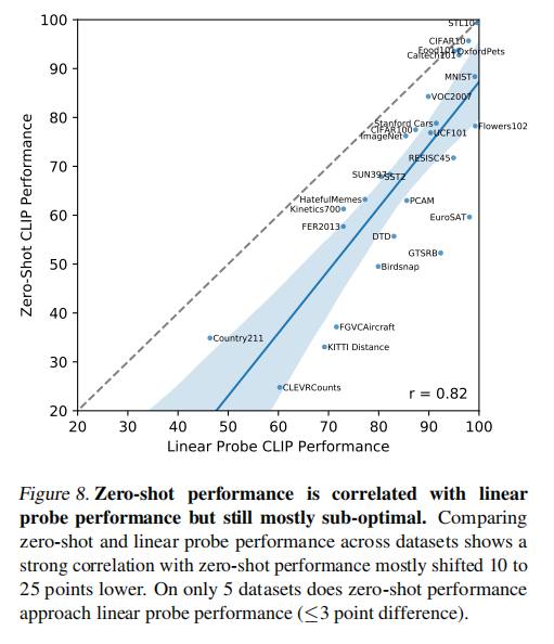
The results in Figure 8 show a strong correlation, but also a consistent gap: the zero-shot classifier is usually 10% to 25% worse than the fully supervised one. This is actually fantastic news. It means that CLIP’s image features are even more powerful than its current zero-shot mechanism can fully exploit. There is still significant headroom to improve the language-based task learning, suggesting that future work on better prompting or other techniques could unlock even more performance from the very same model.

TipA Quick Note: Key Takeaways from the Zero-Shot Performance Analysis

Section 3.1.5 is a deep dive into the practical performance of CLIP’s zero-shot capabilities. The authors go beyond a single headline number and dissect the model’s strengths and weaknesses through a series of clever comparisons. Here are the four main lessons learned:

1. Zero-Shot CLIP is a Supervised Learning Competitor.

To establish a meaningful baseline, the authors compared zero-shot CLIP (which sees no training examples for a given task) against a standard, fully supervised classifier trained on top of features from a powerful ResNet-50. The result was stunning: CLIP beat this supervised baseline on 16 out of 27 diverse datasets. This proves that zero-shot transfer is not just a novelty; it is a genuinely powerful and competitive technique, often more effective than training on thousands of task-specific labeled examples.

2. CLIP Has Clear Strengths and Weaknesses.

The model’s performance is not uniform across all tasks. By analyzing the breakdown, we can infer what kind of knowledge was captured during its web-scale pre-training.

• Strengths: CLIP excels at tasks involving general object recognition and, notably, action recognition in videos. The authors speculate this is because its training on natural language (sentences) provided rich supervision for verbs (actions), whereas traditional datasets like ImageNet are heavily biased towards nouns (objects).
• Weaknesses: CLIP struggles on highly specialized and abstract tasks. This includes niche domains like medical imaging (PatchCamelyon) and satellite photo analysis (EuroSAT), as well as abstract tasks like counting objects (CLEVRCounts). This suggests its knowledge is broad but not infinitely deep, and its capabilities are limited by the concepts present in its vast but not all-encompassing training data.

3. A Good Instruction Can Be Better Than a Few Examples.

Perhaps the most counter-intuitive finding is how zero-shot performance compares to few-shot performance. The authors found that, on average, zero-shot CLIP’s performance was equivalent to that of a 4-shot linear classifier trained on its own features. In other words, giving the model a single, well-crafted text prompt is as effective as giving a standard classifier four labeled examples for every single class. The authors reason that a text prompt is a direct and unambiguous way to communicate a concept, whereas a few image examples can be ambiguous, forcing the model to infer the target concept from a noisy signal.

4. There Is Still Room for Improvement.

The authors compared zero-shot CLIP’s performance to a fully supervised classifier trained on CLIP’s own features. This supervised model represents a rough “upper bound” on the quality of the learned features. They found a consistent gap of 10-25% between the zero-shot and fully supervised results. This is actually very promising news. It means that CLIP’s image representations are even more powerful than its current zero-shot mechanism can tap into. The features are excellent; the bottleneck is in translating any arbitrary text prompt into the perfect classifier. This suggests that future improvements in prompt engineering or other zero-shot techniques could unlock even more performance from the existing CLIP model.

TipA Quick Note: What is a “4-Shot Linear Classifier Trained on CLIP’s Features”?

This phrase describes a specific, controlled experiment designed to fairly measure the quality of a model’s learned features and compare different learning paradigms (like zero-shot vs. few-shot). Let’s dissect the term piece by piece.

1. “…on CLIP’s Features” (The Foundation)

This is the most important part. In this experiment, the powerful, pre-trained CLIP model is used as a fixed feature extractor.

• Step 1: You take an image from a downstream dataset (e.g., a picture of a cat from the Oxford Pets dataset).
• Step 2: You feed this image into CLIP’s Image Encoder.
• Step 3: You take the output vector from one of the final layers of the encoder. This vector is the “features”—a rich, numerical representation of the image.

Crucially, during this entire process, the CLIP model itself is frozen. None of its weights are updated or changed. Its only job is to turn images into high-quality feature vectors. The goal of the experiment is to see how good these features are for a new task.

2. “Linear Classifier” (The Tool)

Now that you have a way to get features, you need to use them to make a prediction. The simplest possible way to do this is with a linear classifier.

• What it is: A linear classifier is a very simple model. For each class, it learns a single “weight vector.” To classify a new image, it calculates the dot product between the image’s feature vector and each class’s weight vector. The class with the highest score wins.
• Why use it? A linear classifier has no hidden layers and no complex non-linearities. It’s deliberately “dumb.” It cannot learn new, complex features; it can only draw simple linear boundaries (lines or planes) in the feature space.

This simplicity is exactly why it’s used for this evaluation. If you can get high accuracy on a task using just a linear classifier on top of the frozen features, it’s a very strong signal that the features themselves are powerful and well-organized. It proves that the feature extractor has already done the hard work of separating the different classes in its representation space.

3. “4-Shot… Trained” (The Constraint)

This part describes the tiny amount of data the linear classifier is allowed to learn from. “K-shot learning” (or few-shot learning) means you train your model using only K labeled examples for each class.

So, a “4-shot trained” classifier for the Oxford Pets dataset (which has 37 classes) would be trained as follows:

1. From the entire training set, you randomly select 4 images of Boxer dogs, 4 images of Beagle dogs, 4 images of Persian cats, and so on for all 37 classes.
2. Your entire training dataset consists of just these 4 * 37 = 148 labeled images.
3. You convert these 148 images into 148 feature vectors using the frozen CLIP image encoder.
4. You then train the simple linear classifier on this tiny dataset of 148 labeled feature vectors.

Putting It All Together

So, the phrase “a 4-shot linear classifier trained on CLIP’s features” describes a process:

1. Freeze the powerful CLIP image encoder.
2. Create a tiny training set by taking only 4 labeled examples per class from a new dataset.
3. Use the frozen CLIP encoder to extract feature vectors for these few examples.
4. Train a simple, “dumb” linear classifier on these feature vectors to perform the new task.
5. Finally, evaluate this classifier’s accuracy on the full test set for that dataset.

The surprising result in the paper is that this whole process, which gets to see four examples of each class, achieves roughly the same average accuracy as CLIP’s zero-shot mechanism, which sees zero examples and relies only on a text prompt.

TipA Quick Note: What is a “Fully Supervised Classifier on CLIP’s Features” and Why is it an “Upper Bound”?

After showing that zero-shot CLIP is surprisingly competitive with a 4-shot classifier, the authors perform one final, crucial experiment. They want to answer the question: “What is the absolute maximum performance we can squeeze out of these image features with a simple classifier, if we give it all the data it could possibly want?” This experiment is often called a “linear probe” and it’s a standard method for evaluating the quality of learned representations.

How It Works: The Same Process, Just More Data

The process for this experiment is nearly identical to the “4-shot” experiment we just discussed. The only difference is the amount of data used.

1. Freeze the CLIP Image Encoder: Just like before, CLIP is used as a fixed, off-the-shelf feature extractor. Its weights are not updated.
2. Extract Features for the Entire Training Set: Instead of using just 4 examples per class, you now take the entire available training set for the downstream task (e.g., all ~50,000 training images for CIFAR-10, or all 1.28 million training images for ImageNet). You run every single one of these images through the frozen CLIP encoder to get their feature vectors.
3. Train a Linear Classifier: You then train the same simple linear classifier on this massive dataset of labeled feature vectors.

How it Compares to the 4-Shot Classifier

The comparison between the two experiments is beautifully simple and highlights the power of data.

Experiment	4-Shot Linear Probe	Fully Supervised Linear Probe
Feature Extractor	Frozen CLIP Image Encoder	Frozen CLIP Image Encoder
Classifier Model	Simple Linear Classifier	Simple Linear Classifier
Training Data	4 images per class	ALL available images in the training set

As you can see, the feature extractor and the classifier are identical. The only variable being changed is the number of labeled examples the linear classifier gets to learn from—a tiny handful versus the entire dataset.

Why is this a “Rough Upper Bound”?

This fully supervised linear probe represents the best-case scenario for a linear classifier operating on CLIP’s features.

• It’s an “Upper Bound”…: Because it has access to all the training data, it represents the highest possible accuracy a linear model can achieve on these features. You can’t give it any more information to learn from. Therefore, the performance of this classifier sets a ceiling, or an upper bound, on what we can expect from any other linear method using these features, including the zero-shot classifier.
• …But it’s “Rough”: The authors wisely call it a “rough” upper bound because a more complex, non-linear classifier (e.g., a multi-layer neural network) could potentially achieve even higher accuracy by learning more intricate patterns in the feature space. However, the linear probe is the standard benchmark in the field because it’s a pure test of the features’ “linear separability”—how well-organized they are.

What the 10-25% Gap Tells Us

The authors found that the fully supervised linear probe consistently outperformed the zero-shot classifier by about 10-25%. This is the most important finding of this analysis.

This gap should not be seen as a failure of CLIP. On the contrary, it is incredibly promising. It means that the feature representations learned by CLIP’s image encoder are so good that they contain more information than the zero-shot mechanism can currently access.

Think of it this way:

• The fully supervised performance represents the total amount of “knowledge” stored in the image features.
• The zero-shot performance represents the amount of that knowledge that can be “unlocked” using a simple text prompt.

The gap between them shows that there is still a wealth of knowledge locked away inside the features. This suggests that the CLIP image encoder is even more powerful than its famous zero-shot performance implies, and that future research into better ways of “prompting” or “instructing” the model could close this gap and unlock even more of its true potential.

3.2 Representation Learning

While zero-shot transfer is CLIP’s most unique feature, it’s also important to ask a more conventional question: how good are the raw visual representations that CLIP learns? Are they as powerful as the features learned by state-of-the-art models trained with supervised or self-supervised methods on ImageNet? This section answers that question with a resounding yes.

Why Evaluate with Linear Probes?

The standard way to measure the quality of a model’s learned representations (or “features”) is to perform linear probe evaluation. The process is simple:

1. Freeze the Model: Take the pre-trained model and lock all of its weights. It is no longer allowed to learn.
2. Extract Features: Pass all the images from a downstream dataset (like CIFAR-10) through the frozen model and save the feature vectors that come out of its penultimate layer.
3. Train a Linear Classifier: Train a simple, single-layer linear classifier (like logistic regression) on these frozen features.
4. Measure Performance: The final accuracy of this simple classifier on the test set is taken as a measure of the quality of the original model’s representations. A higher accuracy means the features are more “linearly separable” and thus of higher quality.

The authors choose this method over end-to-end fine-tuning for several reasons:

• It’s a Fairer Test of the Pre-Trained Features: Fine-tuning allows the model to adapt its features to the new dataset, which can mask failures in the original representation. Linear probes are a purer test of the “out-of-the-box” quality of the pre-trained features.
• It’s Directly Comparable to Zero-Shot: As we’ve discussed, CLIP’s zero-shot classifier is itself a linear classifier. This allows for direct, apples-to-apples comparisons between the zero-shot performance and the “best possible” linear performance on the same features.
• It’s More Manageable at Scale: Fairly fine-tuning dozens of different models across dozens of datasets is a computationally massive and complex undertaking. Linear probes are much simpler and faster to run, making a broad, comprehensive comparison feasible.

CLIP vs. The World: A New State of the Art

The authors compare the linear probe performance of their CLIP models against a comprehensive suite of the best publicly available computer vision models. This includes:

• Supervised Models: EfficientNets, Instagram-pretrained ResNeXts, and Google’s BiT models.
• Self-Supervised Models: SimCLRv2, BYOL, and MoCo.

The results, shown in the incredible plots of Figure 10, are a major statement.

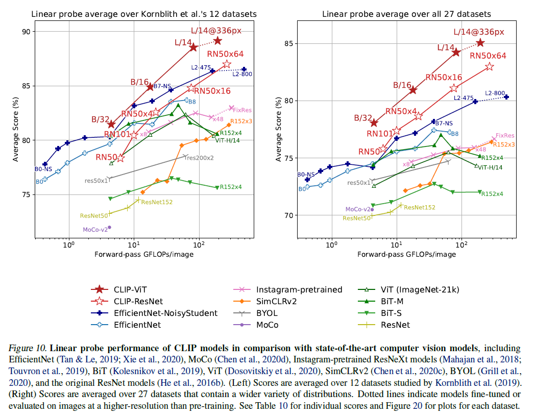
Finding 1: CLIP Models Scale Extremely Well.

When comparing models with similar computational requirements, the smaller CLIP models are competitive but don’t always win. However, the CLIP training approach scales incredibly well. The largest CLIP ResNet model (RN50x64) and the Vision Transformer models decisively outperform the previous best models on the standard 12-dataset benchmark from Kornblith et al. (2019).

The largest model we trained (ResNet-50x64) slightly outperforms the best performing existing model (a Noisy Student EfficientNet-L2) on both overall score and compute efficiency.

Finding 2: Vision Transformers are More Efficient.

The results also confirm a key finding from the original ViT paper: when trained on sufficiently large datasets, Vision Transformers are more compute-efficient than CNNs like ResNet.

We also find that CLIP vision transformers are about 3x more compute efficient than CLIP ResNets, which allows us to reach higher overall performance within our compute budget.

The best overall model, a large Vision Transformer (ViT-L/14), outperforms the best existing model (Noisy Student EfficientNet-L2) by an average of 2.6% across the 12-dataset evaluation suite, solidifying CLIP’s position as the new state-of-the-art in representation learning.

Finding 3: The Broader the Test, the Better CLIP Looks.

The standard 12-dataset benchmark is heavily weighted towards tasks that are similar to ImageNet. The authors argue this might be a form of “selection bias,” and to get a truer sense of general performance, they also evaluate on their broader 27-dataset suite.

On this more diverse set of tasks — which includes OCR, geo-localization, and traffic sign recognition — the benefits of CLIP’s training are even more apparent. The performance gap between the best CLIP model and the previous state-of-the-art widens from 2.6% to 5%. This suggests that CLIP’s pre-training on a diverse set of internet data results in features that are more general and robust than those learned from the more narrow supervision of ImageNet. As shown in Figure 11, CLIP’s features outperform the best ImageNet model’s features on 21 out of the 27 different tasks. This is a powerful demonstration of its superior generalization.

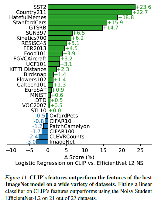
3.3 Robustness to Natural Distribution Shift

For years, deep learning models have been making headlines for achieving “superhuman performance” on benchmarks like ImageNet. However, subsequent research has repeatedly shown that these same models can fail in simple, surprising ways when presented with images that differ even slightly from their training data. This discrepancy is a central problem in modern AI.

What explains this discrepancy? Various ideas have been suggested… A common theme… is that deep learning models are exceedingly adept at finding correlations and patterns which hold across their training dataset… However many of these correlations and patterns are actually spurious and do not hold for other distributions…

A spurious correlation is a pattern that happens to be true in the training data but is not a fundamental truth about the world. For example, if a dataset of cow images mostly shows them in grassy fields, a model might learn that “green pixels at the bottom of the image” is a key feature for identifying a cow. This trick works well for the test set, but the model will fail spectacularly when shown a picture of a cow on a beach.

The authors ask a critical question: is this brittleness an inherent flaw of deep learning, or is it a flaw of the dataset we train them on (i.e., ImageNet)? CLIP provides a perfect opportunity to investigate this.

Measuring Robustness to “Natural Distribution Shift”

To do this, they use a suite of benchmark datasets from a recent paper by Taori et al. (2020) that are specifically designed to test for this kind of failure. These aren’t synthetic corruptions; they are “natural” shifts in the data distribution, created by collecting new images “in the wild.” These include:

• ImageNetV2: A fresh, independent test set for ImageNet collected with the exact same protocol.
• ImageNet-Sketch: Images of objects as black-and-white sketches.
• ObjectNet: Images of objects in unusual orientations (e.g., a chair lying on its side).
• And others…

On these datasets, standard ImageNet models suffer a massive drop in performance. The question is, how does CLIP fare?

Finding 1: Zero-Shot CLIP is Dramatically More Robust

The core hypothesis is that a zero-shot model, by definition, has not been trained on the specific distribution of the test dataset (ImageNet). Therefore, it cannot overfit to its spurious correlations.

Intuitively, a zero-shot model should not be able to exploit spurious correlations or patterns that hold only on a specific distribution, since it is not trained on that distribution. Thus it is reasonable to expect zero-shot models to have much higher effective robustness.

The results, shown in the powerful plot in Figure 13, confirm this intuition in a stunning way. The plot shows ImageNet accuracy on the x-axis and accuracy on the distribution shift datasets on the y-axis.

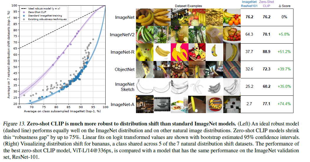
• Standard ImageNet Models: Lie on a line far below the y=x diagonal. A model with 80% accuracy on ImageNet might only get 40% on the robust datasets—a huge “robustness gap.”
• Zero-Shot CLIP Models: Lie on a line much, much closer to the ideal y=x line. They close the robustness gap by up to 75%.

This is a massive finding. It suggests that a significant portion of the brittleness of modern vision models is not an inherent flaw of deep learning, but a direct result of overfitting to the specific biases and spurious correlations present in the ImageNet training set. By learning from a much larger and more diverse dataset of natural language supervision, CLIP learns more robust and generalizable features.

Finding 2: Supervised Fine-Tuning on ImageNet Introduces Brittleness

But is this robustness due to CLIP’s pre-training, or is it simply because it’s a zero-shot model? To test this, the authors perform a fascinating experiment. They take the robust, pre-trained CLIP model and then fine-tune it on ImageNet by training a linear classifier on its features, just as they did in the previous section.

The results, shown in Figure 14, are incredible:

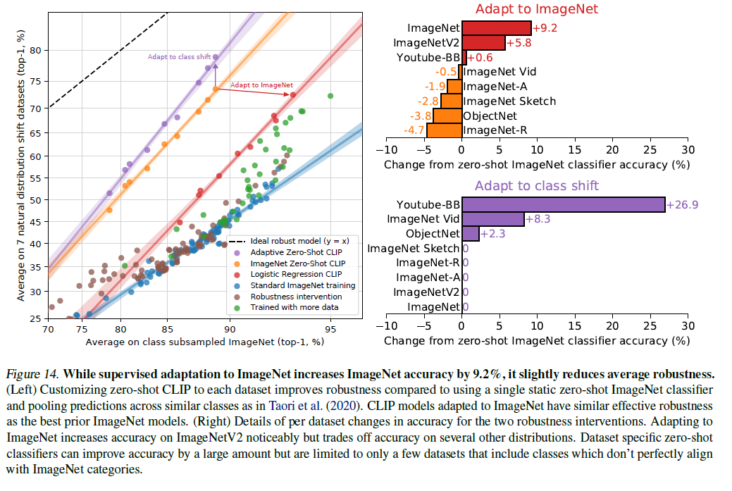
• ImageNet Accuracy: Goes UP by a massive 9.2% (from 76.2% to 85.4%). The model is now even better at the specific task of ImageNet classification.
• Robustness: Goes DOWN. The average accuracy across the seven natural distribution shift datasets slightly decreases.

This is a shocking result. They achieved a 9.2% accuracy gain on the in-distribution task, which corresponds to roughly three years of SOTA progress on ImageNet, and it resulted in zero improvement in out-of-distribution robustness.

This strongly suggests that supervised adaptation to the ImageNet distribution actively encourages the model to learn and exploit the dataset’s spurious correlations. The 9.2% gain in accuracy wasn’t from learning a deeper, more fundamental understanding of the objects; it was from learning the “tricks” needed to do well on the ImageNet test.

Finding 3: Robustness is a Continuum

Finally, the authors investigate how this robustness changes as you move from zero-shot to fully supervised. In Figure 15, they plot the performance of classifiers trained on CLIP’s features with 0, 1, 2, 4, 8… all the way up to all the training examples.

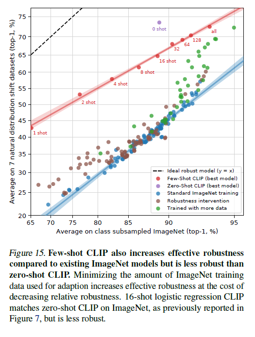
The results show a clear and beautiful trend:

• Zero-shot CLIP is the most robust model.
• As you add more ImageNet training examples (from one-shot to few-shot), the ImageNet accuracy goes up, but the robustness goes down. The model gradually moves away from the ideal y=x robustness line.
• The fully supervised model is the least robust of all.

The conclusion is clear: minimizing the amount of training data from a specific distribution (like ImageNet) leads to higher effective robustness. This is a profound statement about the trade-offs between in-distribution performance and real-world robustness, and it suggests that re-orienting research towards zero-shot and few-shot evaluation is crucial for building more reliable AI systems.

4. Comparison to Human Performance

After demonstrating CLIP’s state-of-the-art performance against other models, the authors introduce a new, more challenging benchmark: human beings. The goal is not just to see who gets a higher score, but to understand the fundamental differences in how humans and machines learn. This comparison reveals a profound gap in sample efficiency and points toward major opportunities for future research.

The Experiment: A Tough, Fine-Grained Challenge

To create a meaningful comparison, the authors chose a difficult, fine-grained visual classification task: identifying 37 different breeds of cats and dogs from the Oxford-IIIT Pets dataset. They then had five human participants perform this task under three different conditions, designed to mirror the machine learning paradigms of zero-shot, one-shot, and two-shot learning.

• Zero-Shot: The humans were given only the list of 37 breed names. They had to classify the images based on their existing prior knowledge of what these breeds look like, without being shown any examples. This is directly analogous to CLIP’s zero-shot setup.
• One-Shot: The humans were shown a single, labeled example image for each of the 37 breeds before they began the classification task.
• Two-Shot: They were shown two example images for each breed.

The Results: A Shocking Gap in Learning Efficiency

The results of this experiment are one of the most insightful parts of the paper. While CLIP’s zero-shot performance on this task is incredibly strong (93.5% accuracy), the way humans learn from examples is radically different and far more efficient.

The key finding is the jump between the zero-shot and one-shot human performance.

Interestingly, humans went from a performance average of 54% to 76% with just one training example per class, and the marginal gain from an additional training example is minimal.

This is a profound difference.

• Humans: A single example image provided a massive +22% boost in accuracy. This suggests that humans are incredibly adept at using one example to resolve their uncertainty. They can effectively “know what they don’t know” and use a single piece of new information to generalize across many different images of the same breed.
• CLIP (and ML Models): As we saw in the previous section (Figure 6), the standard “few-shot” method of training a linear classifier on CLIP’s features shows a slow, gradual improvement with more data. There is no magical jump. The authors even note that for ML models, performance can sometimes drop when going from zero-shot to one-shot because a single, potentially ambiguous example can be a worse learning signal than a clear text description.

The authors’ conclusion is stark:

…it seems that while CLIP is a promising training strategy for zero-shot performance… there is a large difference between how humans learn from a few examples and the few-shot methods in this paper.

Why the Gap? The Power of Prior Knowledge

What explains this vast difference in sample efficiency? The authors speculate that the key is the ability to effectively integrate prior knowledge.

The standard few-shot learning method — training a linear classifier on top of frozen features — is a very simple algorithm. It doesn’t have a sophisticated mechanism for combining the rich, pre-trained knowledge embedded in CLIP’s features with the new information provided by a handful of examples.

Humans, on the other hand, do this automatically. We bring a lifetime of experience and a rich conceptual understanding of the world to any new learning task. We don’t just see a picture of a “Samoyed”; we connect it to our existing knowledge of dogs, fur, animals, and what features are important for distinguishing between them.

This finding suggests that while CLIP has learned an incredible representation of the world, the methods for using that representation in a few-shot setting are still in their infancy. As the authors note, this points to a critical direction for future work: developing better algorithms that can properly integrate a model’s prior knowledge with a few examples to achieve human-like learning efficiency.

A Silver Lining: Shared Difficulty

Interestingly, the experiment also revealed a key similarity: the tasks that are hard for CLIP are also hard for humans. As shown in Figure 16, the specific dog and cat breeds that CLIP had the lowest accuracy on were, by and large, the same ones that humans struggled with. This suggests that both CLIP and humans have captured a meaningful and consistent understanding of the visual similarity between breeds, and their errors are not random but are concentrated on the most genuinely ambiguous cases.

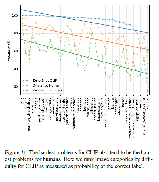
5. Data Overlap Analysis

A major concern for any model pre-trained on a massive, uncurated dataset from the internet is the potential for data leakage or overlap. What if, by chance, some of the images from the downstream evaluation datasets (like the test sets of CIFAR-10 or ImageNet) were also present in the 400 million images used for pre-training?

This is important to investigate since, in a worst-case scenario, a complete copy of an evaluation dataset could leak into the pre-training dataset and invalidate the evaluation as a meaningful test of generalization.

If a model has already “seen the answers” during training, then its high performance on that test set isn’t a measure of its ability to generalize—it’s just a measure of its ability to memorize. Proving that this is not the case is essential for the validity of the paper’s claims.

The Challenge: You Can’t Pre-Filter for Every Possible Test

One way to prevent this is to identify all potential evaluation datasets ahead of time, find any duplicates in your training set, and remove them before you begin training. The authors argue against this approach for a very practical reason:

This has the downside of limiting the scope of benchmarking and analysis. Adding a new evaluation would require an expensive re-train or risk reporting an un-quantified benefit due to overlap.

This is a forward-looking argument. If you pre-filter for today’s 30 benchmarks, you can’t fairly test your model on a new benchmark that someone creates tomorrow without re-training your multi-million dollar model from scratch.

The Solution: Detect, Document, and Analyze

Instead of trying to prevent overlap, the authors choose a more transparent and flexible approach: documenting how much overlap occurs and analyzing how it affects performance.

They developed a sophisticated, three-step procedure to do this for each of their 35 evaluation datasets:

1. Duplicate Detection: They built a custom near-duplicate detection model (detailed in Appendix C) designed to find images in their 400-million-image training set that were visually very similar to the images in each evaluation dataset. This process created two new subsets for each evaluation set:
   • Overlap: The small subset of evaluation images that did have a near-duplicate in the training data.
   • Clean: The large subset of evaluation images that did not.
2. Performance Analysis: They then computed the zero-shot accuracy of CLIP separately on the Overlap and Clean subsets. The main metric of interest is the difference in accuracy between these two (All - Clean). If the model was simply memorizing, its accuracy on the Overlap set should be significantly higher than on the Clean set.
3. Statistical Significance: Because the amount of overlap is often very small, they also performed statistical tests to see if the observed accuracy difference was likely to be real or just due to random chance.

The Results: Overlap is Minimal and Has Almost No Effect

The results of this extensive analysis, presented in Figure 17, provide strong evidence that CLIP’s performance is not a result of memorization.

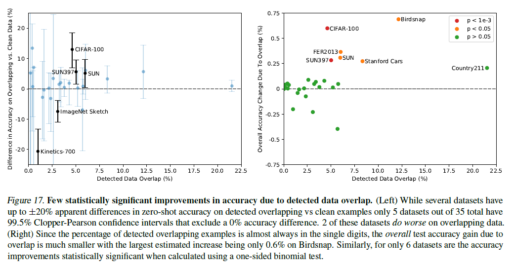
• Overlap is Low: For the vast majority of the datasets, the amount of overlap was very small, with a median of just 2.2% and an average of 3.2%. Some specialized or synthetic datasets had no overlap at all.
• Performance Impact is Negligible: Because the overlap was so small, its effect on the overall reported accuracy was almost nonexistent. For most datasets, the accuracy was shifted by less than 0.1%. The largest “inflation” of accuracy due to overlap was a mere 0.6% on the Birdsnap dataset.
• No Strong Signs of Memorization: Even on the datasets with the most significant overlap (like Country211, which had 21.5% overlap because it was also constructed from Flickr’s YFCC100M dataset), the performance boost was negligible. The authors speculate that even when an image is a duplicate, the text paired with it in the training set is often not relevant to the downstream task (e.g., a photo taken in France might not have the word “France” in its caption).

The authors do acknowledge potential confounders. Their duplicate detector isn’t perfect, and there could be subtle shifts in the type of images that get duplicated (e.g., all-black transition frames in video datasets). However, their findings are consistent with similar analyses done by other researchers (Mahajan et al., 2018; Kolesnikov et al., 2019) on their own large-scale datasets.

Ultimately, this careful and transparent analysis provides strong support for the paper’s main conclusion: CLIP’s remarkable zero-shot performance is a genuine demonstration of generalization, not a trick of memorization.

6. Limitations

While CLIP represents a monumental leap forward, the authors are careful to ground their results by providing a frank and detailed discussion of its limitations. Far from being a perfect, solve-all model, CLIP has clear weaknesses and areas where significant work is still needed.

1. Performance is Still Not State-of-the-Art on Most Tasks

The first and most important limitation is a humbling reality check on performance. While CLIP’s zero-shot performance is often competitive with a supervised ResNet-50 baseline, this baseline is now many years old.

On datasets with training splits, the performance of zero-shot CLIP is on average competitive with the simple supervised baseline of a linear classifier on top of ResNet-50 features. On most of these datasets, the performance of this baseline is now well below the overall state of the art.

In essence, while zero-shot CLIP is a revolutionary capability, it is not (yet) a replacement for a fully supervised, state-of-the-art model trained specifically for a given task. The authors make a sobering estimate of the work that remains:

…we estimate around a 1000x increase in compute is required for zero-shot CLIP to reach overall state-of-the-art performance. This is infeasible to train with current hardware.

This highlights the need for future research into more data-efficient and computationally-efficient training methods. Simply scaling up the current approach is not a viable path to supremacy on every task.

2. Weak Performance on Certain Task Types

As discussed in the zero-shot analysis (Section 3.1.5), CLIP’s performance is not uniform across all types of vision problems. It struggles significantly with several categories of tasks:

• Very Fine-Grained Classification: While it does well on some fine-grained tasks (like food), it struggles with others that require distinguishing between very subtle differences, such as different models of cars, species of flowers, or variants of aircraft.
• Abstract or Systematic Tasks: CLIP is poor at more abstract tasks like counting the number of objects in an image (CLEVRCounts). This suggests its understanding of vision is more about recognizing “what” than “how many.”
• “Un-Googlable” Novel Tasks: For tasks that are truly novel and unlikely to have appeared in its internet-scale pre-training data, CLIP’s performance can be near random. Their example is classifying the distance to the nearest car in a photo, a specialized task from the KITTI self-driving dataset.

3. Poor Generalization to “Truly Out-of-Distribution” Images

While Section 3.3 showed that CLIP is very robust to natural distribution shifts, the authors make it clear that it is still brittle when faced with data that is fundamentally different from its pre-training distribution.

…we’ve observed that zero-shot CLIP still generalizes poorly to data that is truly out-of-distribution for it. An illustrative example occurs for the task of OCR…

CLIP learns a high-quality representation for recognizing text that is digitally rendered, as this is common on the internet. However, its performance on handwritten digits from the MNIST dataset is terrible — achieving only 88% accuracy. This is worse than an “embarrassingly simple baseline of logistic regression on raw pixels.”

This is a critical finding. It shows that CLIP does not solve the underlying problem of brittle generalization in deep learning. Instead, its strategy is to “circumvent the problem” by training on a dataset so massive and varied that it hopes most data will be effectively “in-distribution.” As the MNIST example proves, this is a “naive assumption that… is easy to violate.”

4. The Flexibility Trap: CLIP Can’t Generate Novel Outputs

While CLIP’s zero-shot interface is incredibly flexible for classification, it is still limited to choosing from a predefined set of concepts that you provide as text prompts. It cannot generate novel descriptions for an image it has never seen before.

This is a significant restriction compared to a truly flexible approach like image captioning which could generate novel outputs.

An image captioning model can look at a photo and generate a brand new sentence describing it. CLIP can only tell you which of your proposed sentences is the best match. The authors note that they tried training a captioning model but found it to be far less computationally efficient than the contrastive approach, which is why they chose CLIP’s design. They suggest that future work could explore jointly training a contrastive and a generative model to get the best of both worlds.

5. Data Efficiency is Still Poor

CLIP is not a sample-efficient learner. Its entire premise is the opposite: it compensates for the poor data efficiency of deep learning by leveraging a source of supervision that can be scaled to hundreds of millions of examples. The authors provide a staggering statistic to illustrate this:

If every image seen during training of a CLIP model was presented at a rate of one per second, it would take 405 years to iterate through the 12.8 billion images seen over 32 training epochs.

This highlights that while CLIP is a new paradigm, it does not address the fundamental challenge of creating models that can learn efficiently from a small number of examples, like humans do.

6. Co-Adaptation and Benchmark Haphazardness

Finally, the authors are admirably self-critical about their own evaluation methodology.

• They admit that despite their focus on zero-shot transfer, they repeatedly checked performance on validation sets to guide their research. This is not a “true” zero-shot scenario, where a model is developed in a vacuum and then tested once.
• They also acknowledge that their main 27-dataset evaluation suite was “somewhat haphazardly assembled” and is “undeniably co-adapted with the development and capabilities of CLIP.” In other words, they built a benchmark that, in part, plays to their model’s strengths. They call for the creation of new, standardized benchmarks designed explicitly to evaluate broad, zero-shot transfer capabilities.

7. Broader Impacts

The creation of a powerful, general-purpose technology like CLIP is not a neutral act. It has the potential for both immense benefit and significant harm. In this section, the authors confront these dual-use possibilities head-on, discussing the model’s capabilities, inherent biases, and the challenges it presents for society.

A Double-Edged Sword: The Power of an Arbitrary Classifier

The central capability of CLIP is also its central challenge.

CLIP has a wide range of capabilities due to its ability to carry out arbitrary image classification tasks. One can give it images of cats and dogs and ask it to classify cats, or give it images taken in a department store and ask it to classify shoplifters—a task with significant social implications and for which AI may be unfit.

This perfectly captures the dual-use nature of the technology. The same flexibility that allows a museum to build a tool for art discovery could allow a government to build a tool for surveillance. Furthermore, CLIP makes this power accessible to everyone.

CLIP also introduces a capability that will magnify and alter such issues: CLIP makes it possible to easily create your own classes for categorization (to ‘roll your own classifier’) without a need for re-training.

Before CLIP, deploying a new image classification system for a bespoke task required significant data and expertise. Now, anyone with basic programming skills can define any set of classes they can imagine in plain text and instantly deploy a classifier. This “democratization” of capability is powerful, but it also lowers the barrier for misuse and introduces challenges similar to those seen with large-scale generative models like GPT-3, where the full range of a model’s capabilities (and potential harms) only becomes clear after extensive testing and real-world interaction.

Characterizing Inherited Social Biases

Because CLIP is trained on a massive, unfiltered dataset of image-text pairs from the internet, it inevitably learns and reflects the biases present in that data. The internet is a reflection of society, warts and all, and the model internalizes these associations.

Our bias tests represent our initial efforts to probe aspects of how the model responds in different scenarios, and are by nature limited in scope.

The authors conduct a series of probes to begin to characterize these biases. Using the FairFace benchmark for demographic classification and other exploratory tests, they find significant and concerning issues (which are detailed in Section 7.1 of the paper):

• Denigration and Harmful Associations: The model learns to associate certain demographic groups with harmful concepts. For example, when given crime-related labels like “thief” or “criminal,” the model misclassifies male images at a higher rate than female images. More troublingly, it misclassifies images of Black people into non-human categories (like “gorilla”) at a significantly higher rate than other races.
• Performance Disparities: The model’s accuracy on tasks like gender classification is not uniform across all demographic groups.
• Class Design Sensitivity: The authors show that these biases are highly sensitive to “class design”—the specific words one chooses for the labels. Adding the label “child” to a set of classes, for instance, drastically reduces the number of young people who are misclassified with crime-related labels. This shows how easily a developer’s choices can either amplify or mitigate the model’s inherent biases.

These tests are not comprehensive, but they are a crucial first step. They demonstrate that CLIP, like any model trained on societal data, is not a neutral observer but an active participant in perpetuating social biases. This necessitates careful analysis and mitigation before any real-world deployment.

The Challenge of Surveillance

The authors explicitly address the use of CLIP’s capabilities for surveillance. Many of the tasks CLIP learns to perform—from action recognition and object classification to geo-localization and facial emotion recognition—have direct applications in surveillance.

While they argue that CLIP is not ideally designed for many common surveillance tasks (like object detection) and that its performance may not be competitive with specialized, supervised models, they acknowledge a key risk:

…CLIP and similar models could enable bespoke, niche surveillance use cases for which no well-tailored models or datasets exist, and could lower the skill requirements to build such applications.

This is the core danger. CLIP’s flexibility makes it a powerful tool for creating novel, highly specific surveillance systems “on the fly,” for which no commercial solutions or dedicated datasets currently exist.

The authors’ analysis in this section is a model of responsible research. They do not shy away from the negative potential of their work. Instead, they proactively investigate it, quantify it where possible, and call on the broader AI community to develop more robust testing schemes to better characterize the capabilities and biases of these powerful general-purpose models.

8. Related Work

No research happens in a vacuum. In this section, the authors meticulously map out the surrounding intellectual landscape to clarify what CLIP is, what it isn’t, and how it builds upon decades of prior work. They situate their contribution not as a single, isolated invention, but as a powerful synthesis of ideas from multiple fields.

A Broad Intellectual Heritage in NLP

First, the authors make a bold and expansive claim, arguing that the idea of “natural language supervision” is the bedrock of nearly all of modern NLP.

Any model that leverages written, spoken, signed or any other form of human language as part of its training signal is arguably using natural language as a source of supervision. This is an admittedly extremely broad area and covers most work in the field of distributional semantics including topic models…, word, sentence, and paragraph vectors…, and language models…

They are connecting CLIP to the core principle of distributional semantics: the idea that the meaning of a word (or sentence) can be learned from the contexts in which it appears. This is the foundational concept behind everything from Word2Vec to GPT-3. By framing their work this way, they are claiming that CLIP is essentially an application of this core NLP principle to the visual domain.

The Core Task: Text-Image Retrieval

More specifically, CLIP’s pre-training objective is a form of text-image retrieval. This is a long-standing subfield of computer vision dedicated to finding relevant images for a given text query, and vice versa. The authors acknowledge a rich history of work in this area, which evolved from predictive objectives (trying to predict words) to learning joint multi-modal embedding spaces—the “shared concept space” that is central to CLIP’s design. CLIP’s primary contribution to this specific field is not a fundamentally new algorithm, but rather the successful application of these existing contrastive learning principles at an unprecedented scale.

A Close Cousin: “Webly Supervised Learning”

CLIP is closely related to another popular paradigm called webly supervised learning. This approach involves:

1. Choosing a class name (e.g., “tiger”).
2. Using that name as a query in an image search engine.
3. Using the resulting images as training examples, with the query (“tiger”) as the label.

While this also uses internet-scale data, the authors draw a crucial distinction:

However CLIP only uses full text sequences co-occuring with images as supervision rather than just the queries, which are often only a single word or short n-gram.

This is a critical difference in the richness of the supervision signal. A webly supervised model learns from the pairing [image] -> "tiger". CLIP learns from the pairing [image] -> "a photo of a Bengal tiger resting in the shade". The full, natural language caption provides a much deeper, more nuanced, and more generalizable learning signal than a single-word label.

The Contemporary Competitors: Complex Vision-Language Models

Finally, the authors differentiate CLIP from a family of powerful, contemporary vision-language (V&L) models like ViLBERT, LXMERT, and Oscar. These models are designed for complex reasoning tasks like Visual Question Answering (VQA).

This line of work focuses on richly connecting vision and language in order to solve complex downstream tasks… These approaches leverage impressively engineered models which combine 3 (or more) pre-trained subsystems…

These models typically use a complex joint attention mechanism, where different regions of the image and different words in the text can directly “attend” to each other through multiple layers of a Transformer. This allows for a very deep, fine-grained fusion of the two modalities.

CLIP is fundamentally different in its approach:

The only interaction in a CLIP model between the image and text domain is a single dot product in a learned joint embedding space.

CLIP intentionally avoids this complex, dense fusion. Its image and text encoders are entirely separate, and their representations only interact at the very end via a simple similarity calculation. This architectural simplicity is a deliberate design choice. While it may be less powerful for intricate reasoning tasks, this simplicity is precisely what makes CLIP computationally efficient enough to be scaled up to a dataset of 400 million images. It represents a trade-off: sacrificing deep fusion for massive scale.

9. Conclusion

In their concluding remarks, the authors succinctly summarize the journey and the destination of their research. They frame their work as a successful test of a grand hypothesis: can the principles that revolutionized Natural Language Processing be successfully transferred to the domain of computer vision?

We have investigated whether it is possible to transfer the success of task-agnostic web-scale pre-training in NLP to another domain. We find that adopting this formula results in similar behaviors emerging in the field of computer vision…

Their answer is a clear and confident “yes.” Just as large language models trained on web text develop a surprising ability to perform a wide range of tasks, so too does CLIP.

The authors recap the core mechanism and its powerful outcome:

In order to optimize their training objective, CLIP models learn to perform a wide variety of tasks during pre-training. This task learning can then be leveraged via natural language prompting to enable zero-shot transfer to many existing datasets.

This is the central narrative of the paper in two sentences. The simple, scalable contrastive objective forces the model to learn a rich, general-purpose understanding of visual concepts. This learned knowledge is intrinsically linked to language, which allows it to be flexibly deployed to new tasks through the powerful and intuitive interface of natural language prompting.

Finally, they offer a concluding thought on the performance and the road ahead:

At sufficient scale, the performance of this approach can be competitive with task-specific supervised models although there is still room for much improvement.

This is a statement of both triumph and humility. They have proven that their approach is not just a novelty but a genuinely competitive method that can rival traditional supervised models on their own turf. However, they also acknowledge that the journey is far from over. As their own “Limitations” section made clear, there are still many tasks where supervised models reign supreme, and future work is needed to continue closing this gap.

In essence, the CLIP paper concludes by establishing a new paradigm for computer vision. By successfully adapting the NLP playbook of large-scale, task-agnostic pre-training, the authors unlocked an unprecedented level of zero-shot generalization, fundamentally changing the way we think about building and interacting with models that can see.