DETR: A Deep Dive into End-to-End Object Detection with Transformers

For years, the world of object detection has been dominated by complex, multi stage pipelines. Models like Faster R-CNN and YOLO, despite their success, rely on hand tuned components like anchor boxes and non maximum suppression to function. In 2020, researchers from Facebook AI introduced DETR (DEtection TRansformer), a groundbreaking model that reframes the task entirely. It treats detection as a direct set prediction problem, leveraging the power of transformers to create a truly end to end system. In this post, we will take a detailed, section by section look at the paper to understand how this elegant approach works and why it represents a significant leap forward for the field.
Abstract
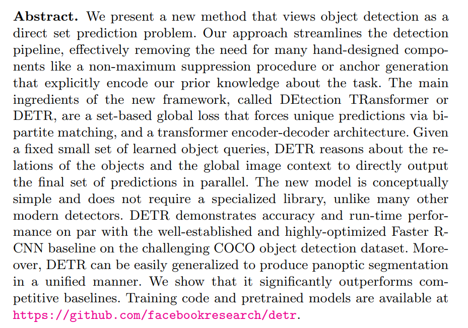
The abstract lays out the entire story of DETR in a few short sentences. It tells us what the core problem is with existing methods, what DETR’s new approach is, what its key components are, and why it matters. Let’s start with the central idea.
We present a new method that views object detection as a direct set prediction problem. Our approach streamlines the detection pipeline, effectively removing the need for many hand-designed components like a non-maximum suppression procedure or anchor generation…
To appreciate why this is so significant, we first need to understand the “old” way of doing things. For years, leading object detectors like Faster R-CNN, SSD, and YOLO have treated object detection as an indirect problem. Instead of directly predicting the final bounding boxes, they follow a multi-stage process:
- Generate massive amounts of proposals: They start by creating thousands of candidate bounding boxes. In some models, these are called anchor boxes, which are predefined boxes of various sizes and aspect ratios tiled across the entire image. The model’s job is not to find a box from scratch, but to slightly adjust (regress) these anchors and classify whether they contain an object.
- Filter the duplicates: This initial step inevitably produces many redundant, overlapping detections for the same object. To clean up this mess, a post-processing step called Non-Maximum Suppression (NMS) is required. NMS is a hand-designed algorithm that keeps the box with the highest confidence score and throws away any other boxes that overlap with it above a certain threshold.
This pipeline, while effective, is complex. Its performance depends heavily on the careful tuning of these components: How many anchors should you use? What should their sizes and aspect ratios be? What is the right overlap threshold for NMS?
DETR’s core contribution is to eliminate this entire pipeline. By framing object detection as a direct set prediction problem, it builds a model that outputs the final, unique set of objects in a single pass. No anchors, no NMS, no complex post-processing.
So, how does it achieve this? The abstract highlights two main ingredients:
The main ingredients of the new framework… are a set-based global loss that forces unique predictions via bipartite matching, and a transformer encoder-decoder architecture.
Let’s quickly define these two concepts.
- Transformer Encoder-Decoder Architecture: Originally developed for machine translation in NLP, the Transformer is a neural network architecture built on self-attention mechanisms. Unlike Convolutional Neural Networks (CNNs) that process information locally, attention allows the model to weigh the importance of all other elements in the input when processing a single element. In computer vision, this means the model can reason about the entire image at once, understanding the global context and the relationships between objects. This global reasoning is key to avoiding duplicate predictions naturally.
- Set-Based Global Loss with Bipartite Matching: This is the clever training strategy that makes direct set prediction possible. The model outputs a fixed-size set of predictions (e.g., 100 boxes). During training, we need a way to compare this predicted set to the ground-truth set of objects in the image. Since the order of predictions doesn’t matter, DETR uses the Hungarian algorithm to find the best one-to-one matching (a bipartite matching) between the predicted and ground-truth boxes. Once each prediction is uniquely assigned to a ground-truth box, a loss is calculated and the model is updated. This forces the model to learn to produce unique, accurate predictions for each object.
The abstract concludes by stating that this conceptually simple model achieves performance on par with a highly optimized Faster R-CNN baseline on the challenging COCO dataset. It also mentions that the architecture is flexible and can be easily extended to more complex tasks like panoptic segmentation, which we’ll explore later.
In essence, the abstract presents DETR as an elegant and powerful alternative to the complex, hand-tuned pipelines that have long dominated object detection.
At the heart of DETR’s training process is a concept from graph theory called bipartite matching, which is used to solve the assignment problem.
Imagine you have two distinct groups of items. For example, a group of job applicants and a group of open job positions. You want to assign each applicant to exactly one job in the most optimal way possible. This is an assignment problem.
A bipartite matching is the formal way to solve this. The two groups of items (applicants and jobs) are the two sets of nodes in a “bipartite graph”. A “matching” is a set of connections between the two groups such that no item is connected to more than one other item.
In the context of DETR:
- Set A is the fixed-size set of
Npredictions made by the model. Each prediction consists of a class label and a bounding box. - Set B is the set of
kground-truth objects in the image. (To make the sets equal in size, this set is padded withN-k“no object” slots).
The goal is to find the best possible one-to-one assignment between the model’s predictions and the actual objects. To do this, we first calculate a “cost” for every possible pairing. This cost measures how dissimilar a predicted box is from a ground-truth box, considering both the class prediction and the box coordinates.
The Hungarian algorithm is then used to find the assignment that minimizes the total cost across all pairs.
Why is this so important? This matching process enforces a unique prediction for each ground-truth object. By finding this optimal matching before calculating the loss, DETR forces the model to learn to produce a clean, duplicate-free set of predictions from the very beginning. It’s the mechanism that allows DETR to get rid of Non-Maximum Suppression (NMS).
1. Introduction
Setting the Stage: Why Object Detection Needed a Rethink
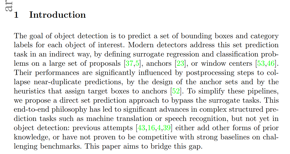
The authors open by clearly stating the fundamental goal of object detection: to predict a set of items, where each item consists of a bounding box and a category label. The key word here is “set”. A set is an unordered collection of unique elements. However, as the authors immediately point out, this isn’t how leading models have historically approached the task.
Modern detectors address this set prediction task in an indirect way, by defining surrogate regression and classification problems on a large set of proposals [37,5], anchors [23], or window centers [53,46].
This sentence masterfully summarizes the core issue with the pre-DETR status quo. Let’s break down what “indirect” and “surrogate” mean in this context.
Instead of directly predicting the final set of objects, models like Faster R-CNN work on a substitute, or surrogate, task. They start by generating thousands of pre-defined bounding boxes, known as anchors or proposals. Think of these as a dense grid of “best guesses” laid over the image. The model’s job is then twofold:
- Classification: For each anchor, classify whether it contains an object or is just background.
- Regression: For each anchor that contains an object, slightly adjust its coordinates (height, width, x/y position) to better fit the ground-truth object.
This indirect approach creates two significant downstream problems, which the authors highlight:
Their performances are significantly influenced by postprocessing steps to collapse near-duplicate predictions, by the design of the anchor sets and by the heuristics that assign target boxes to anchors [52].
First, because you start with thousands of anchors, you inevitably get multiple, slightly different predictions for the same object. This requires a hand-designed post-processing step called Non-Maximum Suppression (NMS) to filter out these duplicates. Second, the entire system’s performance is sensitive to the initial design of the anchors and the “heuristics” (i.e., the rule-based methods) used to match them to ground-truth objects during training. This introduces a lot of complexity and extra hyperparameters that need to be tuned.
DETR’s proposal is to get rid of this entire convoluted process. The authors frame their work as bringing the end-to-end philosophy to object detection. This philosophy, which has been incredibly successful in fields like machine translation and speech recognition, means creating a single, unified model that goes directly from the raw input (the image) to the final output (the unique set of objects) with no intermediate, hand-designed steps.
They conclude by acknowledging that others have tried this before, but that those attempts were not competitive with the highly optimized traditional detectors. The stated goal of this paper is to “bridge this gap” by introducing a model that is both end-to-end and high-performing.
In object detection, regression refers to the task of predicting the continuous numerical values that define a bounding box: its position (like x and y coordinates) and its size (width and height).
The term surrogate means “substitute” or “proxy”. So, surrogate regression is an indirect approach where the model doesn’t predict the final bounding box coordinates directly. Instead, it predicts corrections or offsets relative to a predefined starting point.
Let’s consider the most common starting point: an anchor box.
The Direct Approach (what DETR does): The model is asked, “What are the absolute coordinates of the object in the image?” It might output
(x=0.5, y=0.5, w=0.2, h=0.3)which directly defines the box’s location and size relative to the image.The Surrogate Approach (what Faster R-CNN does): The model is given a fixed anchor box and asked, “How do you need to change this anchor to make it fit the object?” The model’s output isn’t the final coordinates, but a set of deltas, like
(dx=0.1, dy=-0.05, dw=0.2, dh=0.15). These deltas are then used in a formula to adjust the original anchor box’s position and size to get the final prediction.
Why use this indirect method? Historically, it made the learning problem easier. Predicting small adjustments from a good starting guess (the anchor) was more stable and effective for early models than predicting absolute coordinates from scratch. The anchor boxes encode strong prior knowledge about typical object shapes and sizes.
The key takeaway is that surrogate regression is a core part of the complex, multi-stage pipeline that DETR aims to replace. By predicting absolute box coordinates, DETR eliminates the entire machinery of designing, assigning, and regressing from anchors.
Enter the Transformer: A New Architecture for Detection
Having established the limitations of existing pipelines, the authors introduce their solution. They streamline the process by directly tackling the set prediction problem, and they do so by borrowing a powerful tool from the world of Natural Language Processing (NLP).
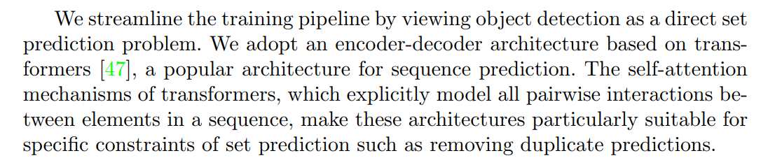
This is the central technical proposal of the paper. Let’s unpack it.
Transformers: This refers to the architecture introduced in the landmark 2017 paper, “Attention Is All You Need.” Transformers revolutionized NLP tasks like machine translation by replacing the recurrent layers (RNNs) common at the time with a new mechanism called self-attention.
Self-Attention: This is the magic ingredient. Unlike a Convolutional Neural Network (CNN) which processes an image through small, local filters, a self-attention mechanism allows the model to consider the entire input at once. When processing a single part of the image (say, a patch corresponding to a cat’s ear), self-attention enables the model to look at every other part of the image (the cat’s tail, a nearby dog, the background) and weigh their importance. This creates a rich, global understanding of the image content.
Modeling Pairwise Interactions: The authors state that self-attention “explicitly models all pairwise interactions.” This is the key to solving the duplicate prediction problem that plagues other models. Because the model can reason about the relationships between all potential objects simultaneously, it can learn that two predictions are targeting the same object. The predictions can effectively “communicate” with each other via the self-attention mechanism, and the model can learn to suppress one of them. This is a learned, dynamic process that replaces the need for a rigid, hand-coded NMS algorithm.
In short, the authors’ central insight is that the global reasoning power of transformers, specifically the self-attention mechanism, is perfectly suited to the task of predicting a set of unique objects. It provides a natural way to enforce the uniqueness constraint without any external post-processing.
Introducing DETR: The DEtection TRansformer
Now, the authors give their new framework a name and succinctly summarize how it works and what makes it different.
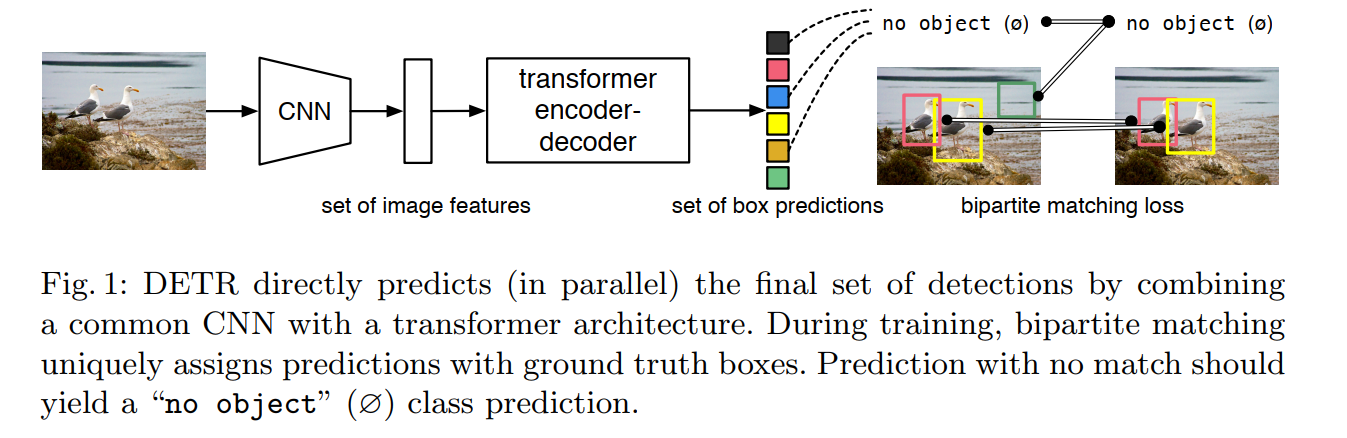
Our DEtection TRansformer (DETR, see Figure 1) predicts all objects at once, and is trained end-to-end with a set loss function which performs bipartite matching between predicted and ground-truth objects.
Here, we get a concise recap of the core mechanics:
- DETR predicts all objects at once: This is a crucial detail. Unlike autoregressive models (like traditional RNNs) that generate outputs one by one in a sequence, DETR decodes all object predictions in parallel. This is a more efficient and holistic approach.
- It uses a set loss with bipartite matching: As we’ve discussed, this is the mechanism that allows the model to be trained on unordered sets of objects. The bipartite matching step creates a unique one-to-one assignment between the predicted and ground-truth boxes, which then allows for a straightforward loss calculation.
Next, the authors hammer home the primary benefit of this design: simplification.
DETR simplifies the detection pipeline by dropping multiple hand-designed components that encode prior knowledge, like spatial anchors or non-maximal suppression.
This is the punchline of the DETR philosophy. The complex, hyperparameter-sensitive machinery of spatial anchors and non-maximal suppression is rendered obsolete. The model learns to perform these functions implicitly through its architecture and training process.
Finally, the authors highlight a significant practical advantage that lowers the barrier to entry for researchers and practitioners.
Unlike most existing detection methods, DETR doesn’t require any customized layers, and thus can be reproduced easily in any framework that contains standard CNN and transformer classes.
This is a bigger deal than it might seem. Many state-of-the-art computer vision models rely on highly specialized code (e.g., custom CUDA kernels) to implement novel layers, making them difficult to reproduce, modify, or deploy. DETR, on the other hand, is built almost entirely from standard, off-the-shelf components: a standard CNN backbone (like ResNet) and a standard Transformer implementation. This makes the architecture remarkably simple and accessible, a quality the authors hope will attract new researchers to the field.
Autoregressive vs. Parallel Decoding: DETR’s Key Architectural Choice
While the idea of end-to-end set prediction wasn’t entirely new, DETR’s approach was fundamentally different from what came before. The authors pinpoint the exact combination of ideas that sets their work apart.
To understand this, we need to define two key terms: autoregressive and non-autoregressive (or parallel) decoding.
Autoregressive Decoding: Think of this as a sequential, step-by-step process. The model predicts the first object, then takes that prediction as input to predict the second object, and so on. It’s like writing a sentence one word at a time, where each new word depends on the ones you’ve already written. This is the natural mode of operation for Recurrent Neural Networks (RNNs), which is why prior attempts at set prediction used them. The downside is that this process can be slow and can’t be easily parallelized.
Non-Autoregressive (Parallel) Decoding: This is what DETR does. It predicts the entire set of objects all at once, in a single forward pass. It doesn’t generate box 1, then box 2, then box 3. It generates
[box 1, box 2, box 3, ..., box N]simultaneously. This is made possible by the Transformer architecture.
So, why is parallel decoding even possible here? The authors provide the answer:
Our matching loss function uniquely assigns a prediction to a ground truth object, and is invariant to a permutation of predicted objects, so we can emit them in parallel.
This is a beautiful and crucial point. The loss function is permutation-invariant, meaning the order of the predictions doesn’t matter. If the model predicts [cat, dog] or [dog, cat], the bipartite matching algorithm will match them to the correct ground-truth objects just the same, and the final loss will be identical. Because the order of the output doesn’t matter for training, the model is free to generate all the outputs at the same time.
This synergy between the permutation-invariant loss and the parallel-decoding capability of the Transformer is the core technical innovation that distinguishes DETR from previous, RNN-based end-to-end detectors.
When the paper says DETR “predicts all objects at once,” it’s referring to a parallel (or non-autoregressive) decoding process. This is a fundamental departure from how sequence-based models, especially older ones, used to work.
The “Old” Way: Autoregressive Prediction
Previous end-to-end approaches, often based on Recurrent Neural Networks (RNNs), generated predictions one by one, in a sequence. This is called an autoregressive model because each prediction depends on the ones that came before it.
Imagine the task is to list the objects in an image. An autoregressive model would:
- Predict the first object:
(cat, [box_coords_1]). - Feed the information about the predicted
catback into the model. - Based on the image and the fact that it just found a cat, predict the second object:
(dog, [box_coords_2]). - Feed information about both the
catanddogback into the model… and so on, until it outputs a special “end of sequence” token.
The key idea is dependency: the prediction for object N is conditioned on the N-1 objects already found. This is inherently sequential and cannot be done in parallel.
The DETR Way: Parallel Prediction
DETR uses a Transformer decoder, which enables a completely different approach. It doesn’t generate predictions sequentially. Instead, it processes a fixed number of “slots” or “queries” all at the same time.
Here’s a simplified view of how it works:
- Input “Object Queries”: The model starts with a fixed-size set of
Nlearned embeddings, called object queries. Let’s sayN=100. You can think of these as 100 empty “slots” waiting to be filled with information about potential objects. - Parallel Processing: The Transformer decoder takes all 100 object queries as input and processes them simultaneously. During this process, each query:
- Extracts information from the entire image (via encoder-decoder attention).
- Communicates with all other 99 queries to understand what other objects are being detected (via self-attention). This is how it learns to avoid making duplicate predictions.
- Final Output: After passing through the decoder, each of the 100 output slots is independently passed through a small feed-forward network to produce a final prediction: either a
(class, bounding_box)pair or a “no object” classification.
The crucial difference is that the prediction for slot #5 does not depend on the final output of slot #4. They are all computed in a single forward pass, reasoning about each other’s existence through the internal self-attention mechanism, not through a sequential dependency chain. This makes the architecture highly efficient and conceptually elegant.
Performance, Promises, and Peculiarities
Having laid out the architecture, the authors now preview the results and discuss the nuances of their new model.
We evaluate DETR on one of the most popular object detection datasets, COCO [24], against a very competitive Faster R-CNN baseline [37]. Faster R-CNN has undergone many design iterations and its performance was greatly improved since the original publication. Our experiments show that our new model achieves comparable performances.
This is a statement of confidence. The authors aren’t comparing DETR to an outdated model; they are benchmarking it against a modern, highly-optimized version of Faster R-CNN, the long-reigning champion of two-stage object detectors. Achieving “comparable performance” right out of the gate with a completely new paradigm is a significant achievement.
However, the overall performance score doesn’t tell the whole story. The authors provide a more detailed breakdown of DETR’s specific strengths and weaknesses:
More precisely, DETR demonstrates significantly better performance on large objects, a result likely enabled by the non-local computations of the transformer. It obtains, however, lower performances on small objects. We expect that future work will improve this aspect in the same way the development of FPN [22] did for Faster R-CNN.
This is a critical insight into how DETR “sees” the world.
- Strength on Large Objects: The Transformer’s self-attention mechanism processes the entire image globally. This allows it to easily see and reason about large objects that span a significant portion of the image, something that can be challenging for CNNs which build up features from local receptive fields.
- Weakness on Small Objects: This is the model’s primary limitation at the time of publication. The authors astutely draw a parallel to the history of Faster R-CNN, which also initially struggled with objects at different scales. That problem was largely solved by the introduction of the Feature Pyramid Network (FPN), which allowed the model to use features from different layers of the CNN to detect objects of various sizes. The authors suggest that a similar multi-scale feature engineering approach could likely solve this issue for DETR in the future.
The authors also flag that training this new model isn’t quite the same as training a conventional detector.
Training settings for DETR differ from standard object detectors in multiple ways. The new model requires extra-long training schedule and benefits from auxiliary decoding losses in the transformer.
This is an important practical note. Transformers are notoriously data-hungry and often require longer training schedules to converge compared to CNNs. Additionally, the authors mention using auxiliary losses, a training trick where the loss function is applied at the output of every decoder layer, not just the final one. This provides a richer, more direct supervisory signal deep within the network, helping the complex architecture learn more effectively.
Finally, they showcase the flexibility and power of the DETR framework beyond simple object detection.
The design ethos of DETR easily extend to more complex tasks. In our experiments, we show that a simple segmentation head trained on top of a pre-trained DETR outperfoms competitive baselines on Panoptic Segmentation…
This is a powerful demonstration of the model’s capabilities. Panoptic Segmentation is a challenging task that unifies object detection (for “things” like cars, people) and semantic segmentation (for “stuff” like sky, road). The fact that a standard DETR model can be adapted to this task by simply adding a small segmentation “head”—and that it achieves excellent results—proves that the core architecture is learning rich, general-purpose visual representations. It’s not just a specialized box-finder; it’s a powerful vision backbone.
3. The DETR Model
3.1 Object Detection Set Prediction Loss
The central challenge for DETR is this: the model outputs a fixed-size set of N predictions, but the ground truth for an image contains a variable number of objects, k. How do you compare these two sets in a way that is differentiable and encourages the model to learn?
DETR infers a fixed-size set of N predictions, in a single pass through the decoder, where N is set to be significantly larger than the typical number of objects in an image.
First, the architecture is designed to always output a fixed number of predictions, N (the paper uses N=100). This N is chosen to be larger than the maximum number of objects you’d expect to find in any single image. For an image that only contains, say, 3 objects, the ground truth is conceptually padded with N-3 “no object” (∅) slots. This way, we always have two sets of the same size to compare: the N predictions and the N (padded) ground truth objects.
The loss calculation is a clever two-stage process:
- First, find the best possible one-to-one matching between the model’s
Npredictions and theNground-truth objects. - Second, compute the loss for these specific matched pairs.
Stage 1: The Optimal Bipartite Matching
This first stage is all about solving the assignment problem. We have two sets, and we need to find the optimal pairing between them.
To find a bipartite matching between these two sets we search for a permutation of N elements σ ∈ SN with the lowest cost: ô = arg min σ∈SN ΣNi=1 Lmatch(yi, ŷσ(i))
This looks complex, but the idea is intuitive. We are searching for the permutation σ (an ordering of the predictions) that minimizes the total matching cost. This is done efficiently using the Hungarian algorithm.
The key is the pair-wise matching cost, L_match. This cost function evaluates how “good” a match is between a single ground-truth object y_i and a single predicted object ŷ_σ(i). The cost is designed to be low if:
- The class prediction is accurate: The model is highly confident in the correct class (e.g., predicting “cat” with 98% probability for a ground-truth cat).
- The bounding boxes are similar: The predicted box and the ground-truth box have a high degree of overlap and similarity. The paper uses a combination of L1 loss and Generalized IoU (GIoU) loss for this, which we’ll cover shortly.
The Hungarian algorithm takes in the cost matrix of every possible prediction-to-ground-truth pairing and returns the best one-to-one assignment—the one with the lowest total cost. This step is a direct replacement for the complex, heuristic-based assignment rules that traditional detectors use to match anchors to ground-truth objects.
Stage 2: The Hungarian Loss
Once the optimal matching ô has been found, calculating the final loss is straightforward. We now have N well-defined pairs of (ground_truth, prediction).
The second step is to compute the loss function, the Hungarian loss for all pairs matched in the previous step. We define the loss similarly to the losses of common object detectors…
The final loss, L_Hungarian, is a sum over all N pairs. For each pair, the loss is a combination of:
- A negative log-likelihood for the class prediction: This is a standard classification loss that penalizes incorrect class predictions.
- A bounding box loss: This is a regression loss that penalizes inaccurate box coordinates. This loss is only applied for pairs where the ground truth is a real object (not the “no object” class).
The authors also note a practical detail: they down-weight the classification loss for pairs matched to the “no object” class. This is because most of the N=100 predictions will be assigned to “no object,” and this weighting prevents the model from becoming lazy and only learning to predict background. It’s a standard technique to handle class imbalance.
In summary, this elegant two-step process—first match, then compute loss—is what enables DETR to be trained end-to-end on unordered sets of objects, forming the foundation of its entire design.
3.2 The DETR Architecture
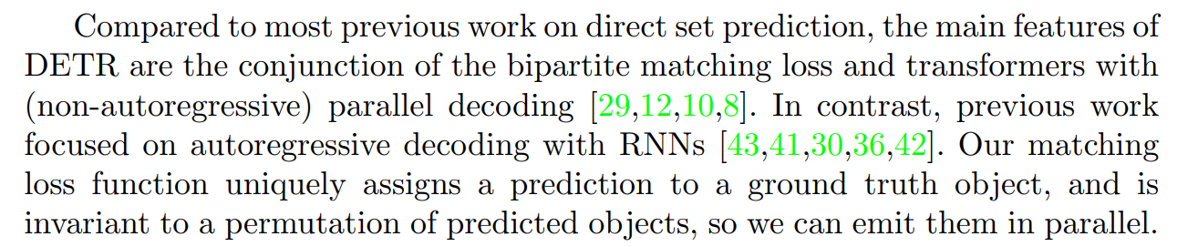
The DETR architecture is surprisingly elegant and can be broken down into three main components, as shown in Figure 2 of the paper.
The overall DETR architecture is surprisingly simple… It contains three main components…: a CNN backbone to extract a compact feature representation, an encoder-decoder transformer, and a simple feed forward network (FFN) that makes the final detection prediction.
This simple, modular design is one of DETR’s greatest strengths. It reuses well-established building blocks in a novel combination. Let’s look at each part in detail.
The Backbone: Feature Extraction
Like most modern computer vision models, DETR starts with a standard Convolutional Neural Network (CNN) backbone.
Backbone. Starting from the initial image… a conventional CNN backbone generates a lower-resolution activation map
f.
- Purpose: The backbone’s job is to act as a feature extractor. It takes the input image (e.g., 800x800 pixels with 3 color channels) and processes it to produce a rich feature map. This map has a smaller spatial resolution (e.g., 25x25) but a much greater channel depth (e.g., 2048 channels). Each “pixel” in this feature map is a high-dimensional vector that represents a specific region of the original image, encoding complex visual patterns like textures, edges, and parts of objects.
- Implementation: The authors use a standard ResNet model, a common and powerful choice for a vision backbone.
The Transformer Encoder: Global Context Reasoning
This is where DETR starts to diverge from traditional detectors. The features from the CNN are passed into a Transformer encoder.
Transformer encoder. … The encoder expects a sequence as input, hence we collapse the spatial dimensions of [the feature map] into one dimension… Since the transformer architecture is permutation-invariant, we supplement it with fixed positional encodings that are added to the input of each attention layer.
- Purpose: The encoder’s goal is to enrich the features from the CNN with global context. It needs to understand the relationships between different objects and parts of the image. For example, it might learn that a feature representing a “person” is often found near a feature representing a “bicycle.”
- Mechanism:
- Flattening: The 2D spatial grid of features from the CNN is “flattened” into a 1D sequence. For a 25x25 feature map, this creates a sequence of 625 feature vectors.
- Positional Encodings: A standard Transformer is permutation-invariant—if you shuffle the input sequence, the output is just a shuffled version of the original. This is a problem for images, where the spatial location of features is critical. To solve this, positional encodings are added to each feature vector in the sequence. These are fixed (not learned) vectors that encode the original
(x, y)position of the feature. This allows the model to retain spatial information while processing the data as a sequence. - Self-Attention: The encoder then processes this sequence of (feature + position) vectors using its multi-head self-attention layers. This allows every feature in the image to attend to every other feature, building a globally-aware representation of the entire scene.
The Transformer Decoder: Object Extraction
The output of the encoder (the context-rich feature map) is then passed to the Transformer decoder, which performs the actual object detection task.
Transformer decoder. The difference with the original transformer is that our model decodes the N objects in parallel… Since the decoder is also permutation-invariant, the N input embeddings must be different to produce different results. These input embeddings are learnt positional encodings that we refer to as object queries.
- Purpose: The decoder’s job is to take the global scene representation from the encoder and extract the location and class of each individual object.
- Mechanism: This is arguably the most innovative part of DETR.
- Object Queries: Instead of feeding the decoder the output of the previous time step (as in an autoregressive model), DETR feeds it a fixed set of
Nlearned embeddings called object queries. You can think of these asNempty “slots” or learnable “object finders.” Each query is a vector that is learned during training and will become responsible for finding a specific type of object or an object in a specific region. - Parallel Decoding: All
Nobject queries are passed into the decoder and processed at the same time (in parallel). - Attention: Inside the decoder, two types of attention are at play.
- Self-Attention: The object queries attend to each other. This is crucial for eliminating duplicate predictions. The queries can “communicate” and learn that if one query is already focused on the main person in the image, the others should look for different objects.
- Encoder-Decoder Attention: Each object query also attends to the output of the encoder. This is how the queries “look at” the image’s feature map to gather the information needed to predict an object’s class and bounding box.
- Object Queries: Instead of feeding the decoder the output of the previous time step (as in an autoregressive model), DETR feeds it a fixed set of
The output of the decoder is a set of N embedding vectors, where each vector now contains rich information about a potential object it has found.
Prediction Feed-Forward Networks (FFNs): The Final Output
The final step is to translate the N output embeddings from the decoder into concrete box predictions and class labels.
Prediction feed-forward networks (FFNs). The final prediction is computed by a 3-layer perceptron… The FFN predicts the normalized center coordinates, height and width of the box… and the linear layer predicts the class label using a softmax function.
A single, small FFN (which is shared across all N outputs for efficiency) takes each of the N embeddings from the decoder and passes it through two separate “heads”:
- A classification head: Predicts the class label for the object (e.g., “person,” “car,” or the special “no object” class).
- A regression head: Predicts the four numbers defining the bounding box (center x, center y, width, height), normalized relative to the image size.
Auxiliary Decoding Losses
Finally, the authors mention a helpful training trick.
We found helpful to use auxiliary losses in decoder during training… We add prediction FFNs and Hungarian loss after each decoder layer.
Instead of just applying the main loss function at the very end of the final decoder layer, they apply it after every decoder layer. This provides a stronger, more direct training signal deep inside the network, helping the model converge faster and achieve better results.
4. Experiments
In this section, the authors transition from theory to practice. They lay out the specifics of their experiments, detailing the dataset, training parameters, and model configurations they used to validate DETR and compare it against the formidable Faster R-CNN.
Dataset
The battlefield for this comparison is one of the most widely used and challenging benchmarks in the field.
We perform experiments on COCO 2017 detection and panoptic segmentation datasets… containing 118k training images and 5k validation images. Each image is annotated with bounding boxes and panoptic segmentation. There are 7 instances per image on average, up to 63 instances in a single image… ranging from small to large on the same images.
The COCO (Common Objects in Context) dataset is the standard for a reason. It’s large, diverse, and features images with complex scenes, multiple objects, significant occlusion, and a wide range of object sizes. A model that performs well on COCO is considered robust and effective. The primary metric reported is AP (Average Precision), which provides a comprehensive measure of a detector’s accuracy across various confidence and overlap thresholds.
Technical Details
The authors provide a transparent and detailed account of their training recipe, which is essential for reproducibility.
Optimizer and Learning Rates: They use the AdamW optimizer, a popular variant of Adam that often leads to better generalization. They also use a much lower learning rate for the CNN backbone (
10^-5) compared to the Transformer (10^-4). This is a common fine-tuning technique where the pretrained backbone is adjusted more cautiously than the randomly initialized new components (the Transformer).Backbones: To ensure a fair comparison, they report results using two different ResNet backbones (ResNet-50 and ResNet-101), which are standard choices in the object detection community. They also experiment with a modified version of the backbone (DETR-DC5) that uses dilated convolutions to increase the feature map resolution. This modification is specifically designed to improve performance on small objects, which they earlier identified as a weakness, but it comes at the cost of increased computation.
Data Augmentation: To improve the model’s robustness and its ability to learn global relationships, the authors employ two key data augmentation techniques:
- Scale Augmentation: Images are resized to a range of different scales during training. This helps the model become invariant to the size of objects in the frame.
- Random Crop Augmentation: With 50% probability, a random rectangular patch of the training image is cropped and then resized. This forces the model to detect objects that are only partially visible and helps the Transformer’s self-attention mechanism learn about broader scene context. The authors note that this improves performance by approximately 1 AP point.
Training Schedule: This is a significant point of difference.
For our ablation experiments we use training schedule of 300 epochs… Training the baseline model for 300 epochs on 16 V100 GPUs takes 3 days… For the longer schedule used to compare with Faster R-CNN we train for 500 epochs…
This is an exceptionally long training schedule compared to traditional detectors. An “epoch” is one full pass over the entire training dataset. For comparison, Faster R-CNN is often trained for schedules equivalent to about 12 or 24 epochs. This highlights that Transformers, while powerful, can be very data- and compute-hungry, requiring extensive training to reach their full potential. This trade-off between performance and training cost is an important practical consideration.
4.1 Comparison with Faster R-CNN
The authors are very deliberate in setting up this comparison. They acknowledge that a straightforward, off-the-shelf comparison would be unfair, as the training methodologies for Transformers and CNN-based detectors like Faster R-CNN have evolved differently.
Transformers are typically trained with Adam or Adagrad optimizers with very long training schedules and dropout… Faster R-CNN, however, is trained with SGD with minimal data augmentation… Despite these differences we attempt to make a Faster R-CNN baseline stronger.
To create a fair and challenging baseline, they don’t just use a standard Faster R-CNN. They create an enhanced version, which we can call Faster R-CNN+, by incorporating modern training techniques that are known to boost performance:
- Generalized IoU (GIoU) loss: A more advanced bounding box loss function.
- Long training schedule: They train Faster R-CNN for a much longer 9x schedule (approximately 109 epochs), which is more comparable to DETR’s long schedule.
- Random crop augmentation: They apply the same data augmentation used to train DETR.
This ensures that any performance advantage shown by DETR is not simply due to a better training recipe but is a genuine reflection of its architectural strengths.
The Results: A New Contender Emerges
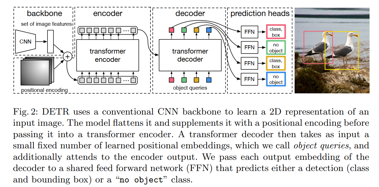
The results are presented in Table 1 of the paper. Let’s analyze the key takeaways by comparing the strongest Faster R-CNN+ model (with a ResNet-101-FPN backbone) to the comparable DETR model (with a ResNet-101 backbone).
…we can conclude that DETR can be competitive with Faster R-CNN with the same number of parameters, achieving 42 AP on the COCO val subset.
At a high level, DETR is right on par with the heavily tuned Faster R-CNN+ baseline. A DETR model with 41M parameters achieves an AP of 42.0, nearly identical to the Faster R-CNN-FPN+ model with 42M parameters that also scores a 42.0 AP. This is a remarkable result for a completely new paradigm. It proves that the end-to-end approach is not just a theoretical curiosity but a viable, high-performance competitor.
However, the headline AP score hides a more interesting story. The real difference lies in what kinds of objects each model excels at. The authors draw our attention to two specific metrics: APS (AP on small objects) and APL (AP on large objects).
The way DETR achieves this is by improving APL (+7.8), however note that the model is still lagging behind in APS (-5.5).
This is the crucial trade-off.
- DETR excels on large objects. The DETR-DC5-R101 model achieves an APL of 62.3, a massive improvement over the strongest Faster R-CNN+’s score of 56.0. This strongly supports the hypothesis that the Transformer’s global self-attention mechanism is superior at understanding and localizing large objects that occupy a significant portion of the image.
- DETR struggles with small objects. The same DETR model scores an APS of only 23.7, significantly lower than Faster R-CNN+’s score of 27.2. This confirms the weakness identified earlier. The single, low-resolution feature map used by the Transformer encoder does not retain enough fine-grained detail to precisely localize small objects.
The authors also show that the modified DETR-DC5 model, which uses a dilated backbone to increase feature resolution, successfully improves APS. However, it still lags behind Faster R-CNN and comes at a high computational cost.
In conclusion, this comparison firmly establishes DETR as a powerful new object detector. While not a “silver bullet” that beats Faster R-CNN on every metric, it demonstrates comparable overall performance and shows a distinct and significant advantage on large objects, validating the power of its global, attention-based reasoning.
4.2 Ablation Studies
Having established that DETR is a competitive model, the authors now ask why. They take their baseline DETR model (ResNet-50 backbone, 6 encoder layers, 6 decoder layers) and conduct a series of experiments, changing or removing one component at a time to measure its impact on performance.
Number of Encoder Layers: The Importance of Global Reasoning
The Question: Is the Transformer encoder, with its global self-attention over the image features, actually necessary?
The Experiment: They train models with a varying number of encoder layers, from 0 (no encoder at all) to 12.
The Result: Removing the encoder entirely causes a significant performance drop of 3.9 AP points. The drop is even more pronounced for large objects (6.0 AP), which are the very objects DETR is best at.
The Conclusion: The encoder is crucial. Its role is to process the raw CNN features and create a globally-aware representation of the scene. By modeling the relationships between all parts of the image, it helps to “disentangle” object instances from each other before the decoder even begins its work. As the authors hypothesize, this likely simplifies the final object extraction and localization task for the decoder.
Number of Decoder Layers: The Power of Iterative Refinement
The Question: Do we really need a deep stack of decoder layers? And if the model is truly end-to-end, can we prove that Non-Maximum Suppression (NMS) is unnecessary?
The Experiment: They analyze the performance of the predictions made after each of the 6 decoder layers. They also test what happens when a standard NMS algorithm is applied to the outputs of each layer.
The Result: The results, shown in Figure 4, are fascinating.
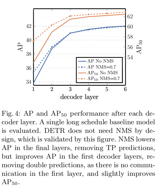
- Performance improves dramatically with each added decoder layer. The output from the first layer is poor, but by the sixth layer, the AP has improved by a massive +8.2 points.
- NMS helps the predictions from the early decoder layers but hurts the predictions from the final layers.
The Conclusion: This is powerful evidence for the effectiveness of the architecture. The first decoder layer acts like a naive detector, producing many duplicate predictions for the same object. In subsequent layers, the self-attention mechanism allows the predictions to “talk to each other,” and the model learns to suppress these duplicates internally. By the final layer, this internal, learned NMS is so effective that applying an external, hand-designed NMS algorithm actually removes correct predictions, lowering the AP. This experiment beautifully validates DETR’s claim of being a truly end-to-end model that does not require NMS.
Importance of FFN
The Question: Are the simple Feed-Forward Networks (FFNs) inside the Transformer blocks important, or is all the magic in the attention layers?
The Experiment: They remove the FFNs from the Transformer, leaving only the self-attention layers.
The Result: Performance drops by 2.3 AP.
The Conclusion: The FFNs are not optional. They can be thought of as 1x1 convolutional layers that follow each attention step. They add computational depth and non-linearity, allowing the model to process the information aggregated by the attention mechanism more effectively.
Importance of Positional Encodings
The Question: How much does the model rely on positional information? What happens if we remove the spatial encodings (from the encoder) or the object queries (from the decoder)?
The Experiment: They test various combinations of removing or modifying the positional encodings.
The Result:
- Completely removing spatial positional encodings causes a catastrophic performance drop of 7.8 AP. The model is lost without a sense of where features are in the image.
- Surprisingly, removing the spatial encodings from the encoder only results in just a small 1.3 AP drop. This suggests the decoder can partially compensate, but having positional information everywhere is still optimal.
- The output positional encodings (the object queries) are absolutely essential and cannot be removed.
The Conclusion: Positional information is critical. The spatial encodings ground the image features in their geometric context, while the object queries act as essential, learnable “anchors” in the output space, giving the decoder a starting point for each prediction.
Loss Ablations
The Question: The bounding box loss is a combination of L1 loss and GIoU loss. Are both needed?
The Experiment: They train models with different components of the box loss turned on and off.
The Result: GIoU loss is the most critical component. A model trained with only GIoU loss performs nearly as well as the full model. In contrast, a model with only L1 loss performs very poorly.
The Conclusion: The Generalized IoU (GIoU) loss, which is scale-invariant, is far more effective for this direct box prediction task than a simple L1 distance loss. The L1 loss provides a small, complementary benefit, but GIoU does the heavy lifting for training the box regression head.
4.3 Analysis
Here, the authors play the role of scientists, probing their trained model to understand its inner workings and test its generalization capabilities.
Decoder Output Slot Analysis: Do Object Queries Specialize?
The core of DETR’s decoder is the set of 100 learned “object queries.” A natural question is: what do these queries actually learn? Are they interchangeable, or do they develop specific roles?
In Fig. 7 we visualize the boxes predicted by different slots for all images in COCO 2017 val set. DETR learns different specialization for each query slot.
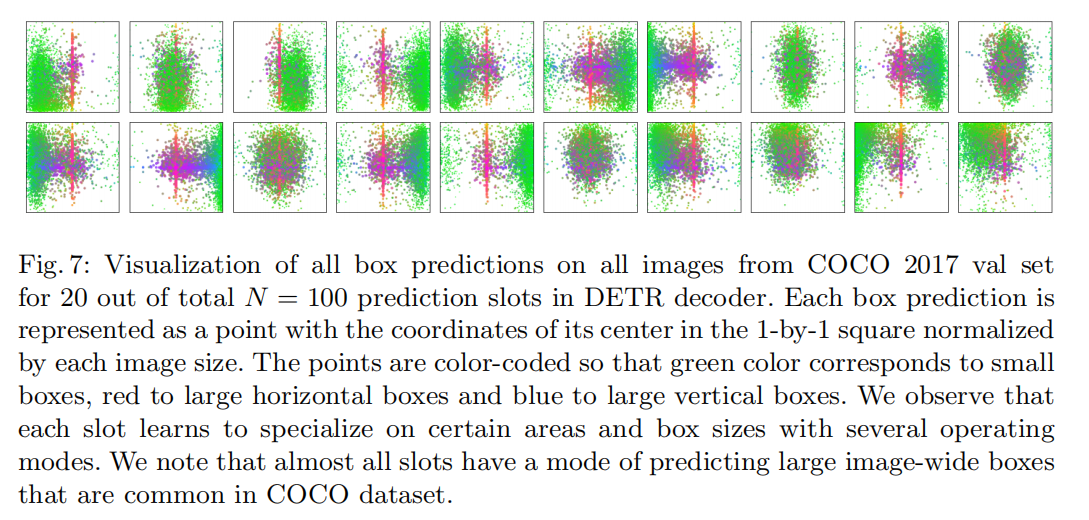
To answer this question, the authors perform a fascinating visualization. For each of the 100 output slots (or queries), they plot the center point of every bounding box it predicted across the entire COCO validation set. The points are color-coded by the size and shape of the box.
The results are striking. The plots are not random scatterings. Instead, each query slot develops a clear specialization.
- One slot might consistently predict small objects near the center of the image.
- Another might specialize in predicting medium-sized, horizontally-oriented objects on the left side.
- A third might focus on large, vertically-oriented objects on the right.
This analysis reveals that the object queries are not just random initializers; they are learned parameters that evolve into a team of specialists. Each query learns to “anchor” its search in a particular spatial area and for a particular box size/shape. This learned, implicit anchoring replaces the hand-designed, explicit anchor boxes of traditional detectors.
The authors also note an interesting pattern:
…almost all slots have a mode of predicting large image-wide boxes… We hypothesize that this is related to the distribution of objects in COCO.
This makes intuitive sense. Many images in COCO are dominated by a single large object. Therefore, it’s a common and important pattern for most queries to learn as a high-probability “mode” of prediction.
Generalization to Unseen Numbers of Instances: The Giraffe Test
A key question for any new model is how well it generalizes to situations it has never encountered in training. The authors devise a clever synthetic experiment to test this.
Some classes in COCO are not well represented with many instances of the same class in the same image. For example, there is no image with more than 13 giraffes in the training set.
What would happen if DETR were shown an image with, say, two dozen giraffes? Would it break down, having never seen such a dense crowd of a single object type? This is a classic “out-of-distribution” test.
We create a synthetic image³ to verify the generalization ability of DETR (see Figure 5). Our model is able to find all 24 giraffes on the image which is clearly out of distribution. This experiment confirms that there is no strong class-specialization in each object query.
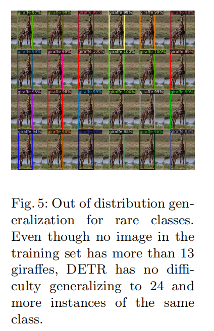
The result is a strong testament to the model’s robustness. Despite never being trained on such an image, DETR successfully detects all 24 giraffes. This implies two important things:
- The model is not overfitting to the object count statistics of the training set. It’s not learning a rule like “there are usually only a few giraffes.”
- The object queries are flexible. They are not hard-coded to find a specific class. The self-attention mechanism between the queries allows them to coordinate dynamically. In essence, the queries can “negotiate” among themselves to say, “I’ve got this giraffe, you handle that one,” ensuring that each object is detected by exactly one query, even in a dense and unfamiliar scene.
This analysis provides powerful evidence that DETR is learning a truly generalizable procedure for object detection, not just memorizing the biases of its training data.
4.4 DETR for Panoptic Segmentation
To truly test the power and flexibility of their new architecture, the authors extend DETR to tackle panoptic segmentation. This is a challenging task that provides a more holistic understanding of a scene than object detection alone. It requires the model to:
- Detect and segment all individual objects (“things” like cars, people, animals).
- Segment all amorphous background regions (“stuff” like sky, road, grass).
- Combine these into a single, unified output where every pixel in the image is assigned both a class label and an instance ID.
This is a perfect test for DETR’s design ethos. The move from object detection to instance segmentation has a famous precedent: Mask R-CNN, which extended Faster R-CNN by adding a simple “mask head” to predict a segmentation mask for each detected bounding box. The DETR authors show they can do the same, but with even greater elegance.
A Simple Extension: Adding a Mask Head
The adaptation is remarkably straightforward. On top of the standard DETR architecture, they add a new prediction head.
…DETR can be naturally extended by adding a mask head on top of the decoder outputs.
For every one of the N object predictions coming out of the Transformer decoder, this new mask head predicts a corresponding binary segmentation mask for that object. The mask head itself is a small FPN-like architecture that uses attention to draw information from the decoder’s object embeddings and the encoder’s image features to generate the pixel-level masks.
Crucially, DETR’s unified set-prediction framework allows for an incredibly clean approach: > We train DETR to predict boxes around both stuff and things classes on COCO, using the same recipe.
Unlike many specialized panoptic segmentation models that have separate architectural pathways for “things” and “stuff,” DETR treats them identically. A patch of grass is just another “object” for the model to predict a box and mask for. This unified view is a natural fit for the set-prediction framework.
The Results: Dominating the “Stuff”
The results, presented in Table 5, show that this simple extension is highly effective. DETR outperforms established methods like PanopticFPN, even when the authors retrain PanopticFPN with the same long schedule and data augmentations for a fair comparison.
But the most insightful result comes from the performance breakdown between “things” and “stuff.”
The result break-down shows that DETR is especially dominant on stuff classes, and we hypothesize that the global reasoning allowed by the encoder attention is the key element to this result.
This is a powerful conclusion that gets to the heart of why the Transformer architecture is so well-suited for vision. “Stuff” classes like “sky,” “road,” or “grass” are often large, amorphous regions that lack strong local textures. A traditional CNN, with its localized receptive fields, can struggle to classify these regions confidently.
DETR’s Transformer encoder, on the other hand, has a global view of the image. The self-attention mechanism can easily see that a large blue region at the top of the image is “sky” by reasoning about its relationship to the “buildings” and “road” below it. This global context reasoning is a massive advantage for understanding the broad, semantic layout of a scene, leading to DETR’s superior performance on “stuff” segmentation.
This experiment solidifies DETR’s status as more than just a clever object detector. It is a powerful and flexible architecture for general scene understanding.
5. Conclusion
The conclusion of the DETR paper provides a concise and confident summary of the work, while also being forward-looking about the new research directions it opens up.
Summary of Contributions
The authors begin by restating their core achievements in a clear and impactful way.
We presented DETR, a new design for object detection systems based on transformers and bipartite matching loss for direct set prediction.
This single sentence encapsulates the two key ingredients: the architecture (Transformers) and the training objective (bipartite matching loss). They emphasize that this combination leads to a new “design,” a fundamental rethinking of the problem.
They then highlight the key results and benefits of this new design:
- Performance: It achieves “comparable results to an optimized Faster R-CNN baseline,” proving its viability.
- Simplicity and Flexibility: It is “straightforward to implement” and “easily extensible to panoptic segmentation,” demonstrating its elegance and power.
- Architectural Advantage: It achieves “significantly better performance on large objects than Faster R-CNN, likely thanks to the processing of global information performed by the self-attention.” This links a specific, measurable result directly back to the core architectural innovation.
Acknowledging the Challenges
Great research doesn’t just celebrate its successes; it also identifies its limitations. The authors are candid about the new set of problems that DETR introduces.
This new design for detectors also comes with new challenges, in particular regarding training, optimization and performances on small objects.
This is a crucial and honest assessment. They acknowledge the three main hurdles that future work on DETR-like models will need to address:
- Training: As noted in the experiments, DETR requires a very long training schedule and can be sensitive to hyperparameter tuning. Making the training process faster and more stable is a key area for improvement.
- Optimization: The computational cost of the Transformer’s self-attention, especially in the encoder, scales quadratically with the number of image features. This can be a bottleneck, and more efficient attention mechanisms are needed.
- Performance on Small Objects: This is the most significant performance limitation identified in the paper. The single-scale, low-resolution feature map from the CNN backbone is not ideal for detecting small objects, and future work will need to incorporate multi-scale features, much like FPN did for Faster R-CNN.
The authors conclude with a hopeful and insightful historical perspective.
Current detectors required several years of improvements to cope with similar issues, and we expect future work to successfully address them for DETR.
This is a perfect closing thought. They remind the reader that models like Faster R-CNN were not perfect when they were first introduced. They were the product of years of iterative refinement and community effort. The authors position DETR not as a final, perfected solution, but as a groundbreaking new foundation upon which the community can build the next generation of object detectors.