A Deep Dive into Feature Pyramid Networks for Object Detection
In the world of computer vision, one of the most persistent challenges is detecting objects that appear at vastly different scales within the same image. A model might easily spot a car filling the frame but completely miss a tiny car in the distance. The classic solution involved creating an image pyramid, resizing the input image into multiple scales and searching for objects at each level. While effective, this approach is computationally expensive, especially for modern deep learning models. In their 2017 paper, Lin et al. from Facebook AI Research introduced the Feature Pyramid Network (FPN), an elegant architecture that provides the benefits of a pyramid representation without the prohibitive cost.
Abstract
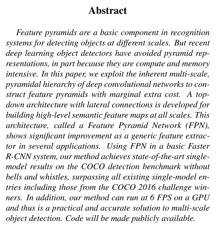
The abstract immediately sets the stage by identifying a fundamental problem in object detection: recognizing objects at various scales. The authors remind us of the classic solution, the feature pyramid, but highlight why modern deep learning models have largely abandoned it: it’s too slow and memory-hungry.
The core insight of the paper is presented as an elegant solution to this dilemma. Instead of building an image pyramid by resizing the input image multiple times, the authors propose to use the pyramid that naturally exists inside a Convolutional Network (ConvNet).
Let’s break that down:
- Inherent Pyramidal Hierarchy: As an image passes through a ConvNet, it goes through a series of layers. Pooling or strided convolutional layers progressively shrink the spatial dimensions of the feature maps. For example, an input of 224x224 might become 112x112, then 56x56, and so on. This creates a natural pyramid of feature maps within the network.
- The Problem with the Natural Pyramid: The issue is that while the final, small feature maps are rich in semantic information (they know what object is present), they have poor spatial resolution (they’ve lost information about exactly where it is). Conversely, the initial, large feature maps have precise spatial information but are semantically weak (they only represent low-level features like edges and textures). Simply making predictions from these different layers doesn’t work well, especially for small objects.
This is where the authors’ key architectural innovation comes in. They propose a Feature Pyramid Network (FPN) that combines the best of both worlds. It uses a “top-down pathway” to carry the strong semantic information from the deep layers back to the shallower layers, and “lateral connections” to merge this with the high-resolution spatial information from those shallower layers. The result is a set of feature maps that are rich in semantic meaning at every single scale.
The authors then state their results in a way that underscores the power and practicality of their method:
- They integrated FPN into a standard Faster R-CNN detector.
- They achieved state-of-the-art results on the challenging COCO benchmark, even beating the winners of the 2016 competition.
- They did this “without bells and whistles,” meaning the improvement comes directly from the FPN architecture itself, not from other common tricks.
- The model runs at 6 FPS, making it a practical and efficient solution.
In essence, the abstract promises a method that delivers the power of a feature pyramid without the high computational cost, solving a long-standing problem in a simple and effective way.
1. Introduction
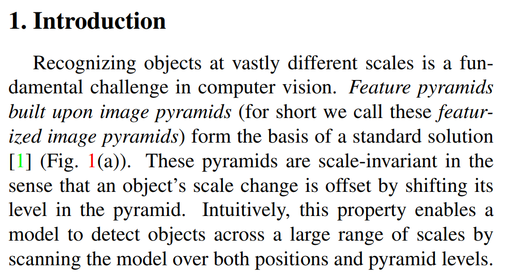
The Fundamental Challenge of Scale
The authors begin by framing the core problem they aim to solve, a classic and difficult one in computer vision: how can a model detect an object regardless of its size in the image? The traditional and intuitive way to solve this is by using an image pyramid. This simply means taking the input image and repeatedly resizing it to create a stack of images at different scales, from large to small.
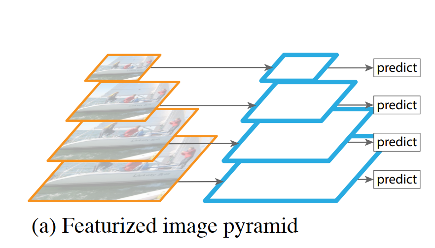
From this image pyramid, a featurized image pyramid is built. As illustrated in Figure 1(a) of the paper, this involves running a feature extractor (in the past, this would have been something like SIFT or HOG; with deep learning, it’s a ConvNet) on each and every level of the image pyramid.
The power of this technique lies in a property called scale-invariance. Imagine a detector trained to find a cat that is 100x100 pixels. If it’s given an image with a tiny 25x25 pixel cat, it will likely fail. But in an image pyramid, that small cat might appear as a 100x100 pixel cat in one of the upscaled versions of the image. Conversely, a giant 400x400 cat might be scaled down to 100x100 in a different level of the pyramid.
The key idea is that the detector only has to be good at recognizing the object at a single, canonical scale. The pyramid structure transforms the problem of handling scale variation into simply choosing the right pyramid level to look at. This is what the authors mean when they say an object’s scale change is “offset by shifting its level in the pyramid.” This robust approach formed the bedrock of many successful object detection systems before the deep learning era.
The Rise of ConvNets and the Compromise of Single-Scale Detection
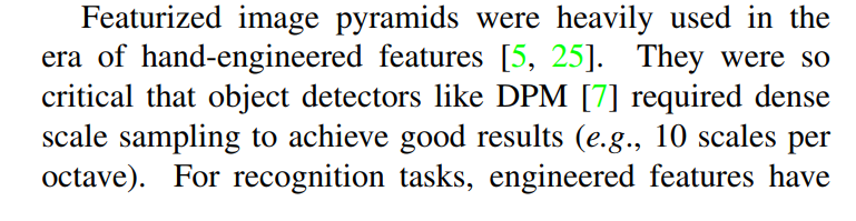
“Featurized image pyramids were heavily used in the era of hand-engineered features [5, 25]. … For recognition tasks, engineered features have largely been replaced with features computed by deep convolutional networks (ConvNets) [19, 20].”
The authors first provide some historical context. Before deep learning, object detectors relied on hand-engineered features like HOG (Histograms of Oriented Gradients) and SIFT (Scale-Invariant Feature Transform). These feature extractors were clever, but not very robust to changes in scale. To get good results, detectors like DPM (Deformable Part Models) had to process the image at many different scales (e.g., “10 scales per octave,” meaning 10 different image sizes just to cover a doubling of object size). This made them powerful but very slow.
Then came the deep learning revolution. ConvNets replaced these hand-engineered features for two key reasons:
- They learn higher-level semantics: Instead of just capturing simple patterns like edges and gradients, ConvNets learn a hierarchy of features. Deeper layers can represent complex concepts like “a wheel” or “an eye,” making them far more powerful for recognition.
- They are more robust to scale variance: Thanks to mechanisms like pooling layers and large receptive fields, a ConvNet can recognize an object even if its size varies a bit.
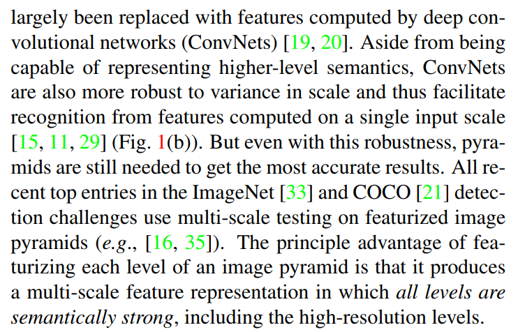
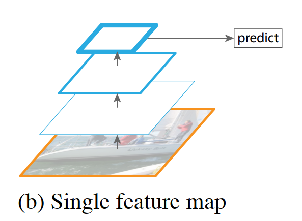
“Aside from being capable of representing higher-level semantics, ConvNets are also more robust to variance in scale and thus facilitate recognition from features computed on a single input scale [15, 11, 29] (Fig. 1(b)). But even with this robustness, pyramids are still needed to get the most accurate results.”
This improved robustness led to a major simplification in object detection architectures. Models like Fast R-CNN and Faster R-CNN abandoned the computationally expensive image pyramid. Instead, they adopted a much faster approach: feed a single, fixed-size image to the ConvNet and extract features from just one of its layers (as shown in Figure 1(b)). This was a practical trade-off, sacrificing some accuracy for a massive gain in speed.
However, the authors deliver a crucial punchline: this trade-off is a compromise. The highest-performing models in top competitions like ImageNet and COCO still use the old-school, slow-and-steady approach of featurized image pyramids at test time. This is strong evidence that, while single-scale detection is fast, it leaves accuracy on the table.
“The principle advantage of featurizing each level of an image pyramid is that it produces a multi-scale feature representation in which all levels are semantically strong, including the high-resolution levels.”
This sentence perfectly captures the “gold standard” that the authors are trying to replicate. When you run a powerful ConvNet on every level of an image pyramid, you get a set of feature maps at different scales. Crucially, every single one of these feature maps is semantically strong, because the full power of the ConvNet was used to create it. The high-resolution feature maps are just as “smart” as the low-resolution ones. This is the ideal scenario, but as we’ll see next, it comes with a heavy price.
The Prohibitive Cost of Image Pyramids
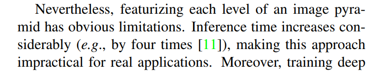
“Nevertheless, featurizing each level of an image pyramid has obvious limitations. Inference time increases considerably (e.g., by four times [11]), making this approach impractical for real applications.”
While using a featurized image pyramid gives the best accuracy, it comes with a crippling downside: it is incredibly slow. Inference time refers to the time it takes for a trained model to make a prediction on a new image. If you build an image pyramid with four different scales, you have to run the entire, massive ConvNet four separate times. This linear increase in computation makes the approach far too slow for real-world applications like autonomous driving or video analysis where speed is essential.
“Moreover, training deep networks end-to-end on an image pyramid is infeasible in terms of memory…”
If inference is slow, training is even worse. In fact, the authors state it is infeasible. During training, a network not only performs a forward pass through the data but also a backward pass (backpropagation) to calculate gradients and update its weights. This requires storing the “activations” (the output feature maps) from every layer in GPU memory. Modern GPUs have a limited amount of memory, and trying to process a whole batch of multi-scale image pyramids at once would cause it to run out of memory almost instantly.
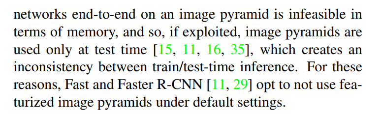
“…and so, if exploited, image pyramids are used only at test time [15, 11, 16, 35], which creates an inconsistency between train/test-time inference.”
Because end-to-end training on an image pyramid is impossible, researchers have relied on a workaround. They train the model on single-scale images (which is memory-efficient) and then, at test time, they apply this model to a multi-scale image pyramid.
This creates a significant problem: a train-test discrepancy. The model is being evaluated in a way it was never trained. It has learned to detect objects at the scale distribution present in the single-scale training images, but it’s being tested on objects at different scales created by the pyramid. This inconsistency can prevent the model from achieving its full potential.
For all these reasons—slow inference, infeasible training, and the train-test discrepancy—the default configurations of influential models like Fast R-CNN and Faster R-CNN abandoned image pyramids entirely in favor of a faster, single-scale approach. This set the stage for a new solution, one that could provide the power of a pyramid without its crippling costs.
The ‘Free’ Pyramid Inside Every ConvNet
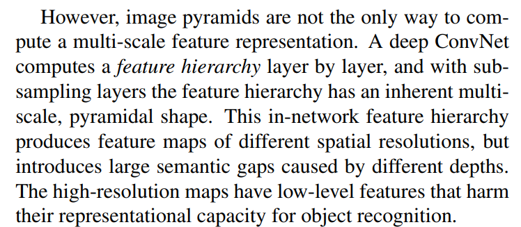
“However, image pyramids are not the only way to compute a multi-scale feature representation. A deep ConvNet computes a feature hierarchy layer by layer, and with subsampling layers the feature hierarchy has an inherent multi-scale, pyramidal shape.”
Having established that building an image pyramid is too expensive, the authors present a powerful alternative that has been hiding in plain sight. Every standard deep ConvNet, like a ResNet or VGG, already contains a pyramid. This is the in-network feature hierarchy.
As an image is processed through a ConvNet, it passes through sequential layers. Some of these layers, like max-pooling or strided convolutions, are subsampling layers. Their job is to reduce the spatial dimensions (height and width) of the feature maps. For example, a 256x256 feature map might become 128x128, then 64x64, and so on, as it gets deeper into the network. This process naturally creates a pyramid of feature maps of decreasing size, all from a single input image and a single forward pass. This pyramid is computationally “free” because the network has to compute these feature maps anyway.
This seems like a perfect solution, but there’s a major catch.
“This in-network feature hierarchy produces feature maps of different spatial resolutions, but introduces large semantic gaps caused by different depths. The high-resolution maps have low-level features that harm their representational capacity for object recognition.”
This is the crucial problem with the “free” pyramid. The different levels of this pyramid are not created equal. There is a large semantic gap between them.
- Shallow Layers (e.g., conv2): These early layers produce large, high-resolution feature maps. However, they are semantically weak. They represent very simple, low-level features like edges, corners, and textures. They have precise location information (“there is an edge here”) but have no concept of what object those edges belong to.
- Deep Layers (e.g., conv5): These final layers produce small, low-resolution feature maps. They are semantically strong. Having processed the entire image through many layers, they represent high-level concepts like “car” or “person.” They know what is in the image, but due to repeated subsampling, they’ve lost precise information about where it is.
Using this pyramid directly for object detection is problematic. If you try to detect small objects using the early, high-resolution layers, you will fail because those layers don’t have strong enough semantic information to actually recognize the object. This is the core challenge the authors are about to solve: how to make every level of this “free” in-network pyramid semantically strong.
A Step in the Right Direction: The Single Shot Detector (SSD)
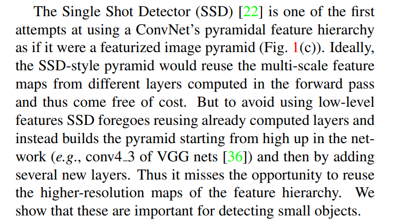
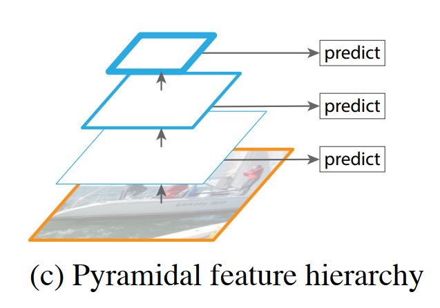
“The Single Shot Detector (SSD) [22] is one of the first attempts at using a ConvNet’s pyramidal feature hierarchy as if it were a featurized image pyramid (Fig. 1(c)).”
Before presenting their own solution, the authors acknowledge a key predecessor: the Single Shot Detector, or SSD. SSD was a clever and influential model that recognized the potential of using the “free” in-network feature pyramid. Instead of making predictions from just one layer (like Faster R-CNN), SSD made predictions from multiple layers at different depths and scales, all within a single forward pass of the network.
This sounds like a great idea, but it ran headfirst into the “semantic gap” problem we just discussed. The SSD authors knew that the early, high-resolution feature maps were semantically weak and not suitable for accurate object classification.
“But to avoid using low-level features SSD foregoes reusing already computed layers and instead builds the pyramid starting from high up in the network (e.g., conv4_3 of VGG nets [36]) and then by adding several new layers.”
SSD’s solution was a compromise. It decided to completely ignore the early, high-resolution layers of the network (like conv2 or conv3) because their features were too primitive. Instead, it started making predictions from a deeper layer (like conv4_3), which already had reasonably strong semantic information. To get feature maps for detecting even larger objects, SSD didn’t use the even deeper layers directly; it appended a new series of smaller convolutional layers to the end of the backbone network.
This is a crucial point. SSD doesn’t reuse the full, existing pyramid. It throws away the bottom, high-resolution levels and builds a new, smaller pyramid on top of the network, as shown in Figure 1(c).
“Thus it misses the opportunity to reuse the higher-resolution maps of the feature hierarchy. We show that these are important for detecting small objects.”
Here, the authors deliver their core critique of SSD’s design. By discarding the high-resolution feature maps from the early layers, SSD handicaps its ability to detect small objects. Small objects require fine-grained spatial information to be located and recognized, and that information is most present in the early layers. SSD’s decision to avoid these layers due to their weak semantics means it pays a heavy price in performance on small objects.
This sets the stage perfectly for the FPN. The authors have identified a clear gap: we need a way to make those high-resolution maps from the early layers semantically strong, so we can use them to accurately detect small objects.
In the context of a ConvNet, the semantic gap refers to the large difference in the meaning of the information carried by low-level and high-level feature maps.
Let’s use a more detailed analogy: imagine an intelligence agency analyzing satellite photos to find enemy tanks.
1. The Low-Level Analyst (Early ConvNet Layers)
This analyst is a junior photo interpreter. Their job is to look at a high-resolution photo and identify very basic shapes and textures.
- What they report: “I see a dark green blob here.” “There is a long, straight line at these coordinates.” “This area has a repeating, metallic texture.”
- Strengths: Their report is incredibly precise spatially. They can give you the exact pixel coordinates of the line or blob. This is high resolution.
- Weakness: Their report has almost no meaning or semantics. The straight line could be a gun barrel, a fence post, or a road. The green blob could be a tank, a bush, or a tent. They have no context. This is semantically weak.
These are the features in conv1 or conv2 of a network. They are great for localization but terrible for recognition.
2. The High-Level Strategist (Deep ConvNet Layers)
This is the senior general who receives reports from hundreds of analysts. They don’t look at the raw photos. Instead, they look at a summary map where information has been processed and condensed.
- What they report: “The enemy is concentrating armor in the northern sector.” “There is a 95% probability of a tank platoon hiding in this forest.”
- Strengths: Their reports are packed with high-level meaning. They understand the concept of a “tank platoon” and “concentrating armor.” This is semantically strong.
- Weakness: Their information is spatially coarse. They know the tanks are somewhere in the northern sector, but they can’t point to the exact tree they are hiding behind. The process of summarizing all the data has lost that fine-grained detail. This is low resolution.
These are the features in conv5 of a network. They are great for recognition but terrible for precise localization.
The Semantic Gap
The semantic gap is the vast difference between the junior analyst’s report and the general’s understanding.
- You can’t just hand the analyst’s report (“there’s a line at pixel X,Y”) to the general. It’s too low-level and lacks the context for making a strategic decision.
- You can’t ask the general to draw a precise box around a tank. They only have the summarized, low-resolution view.
This is the exact problem SSD faced. It couldn’t use the early, high-resolution layers because they were semantically weak (the junior analyst). So, it started its work much higher up the chain of command, where the features were already semantically meaningful (the mid-level officers and the general).
The genius of FPN is that it creates a way for the general’s high-level understanding to flow back down to the junior analyst, giving them the context to understand that the “straight line” they see is actually a gun barrel and the “green blob” is a tank. It enriches the high-resolution maps with high-level semantics, bridging the semantic gap.
The Solution: A Top-Down Pathway with Lateral Connections
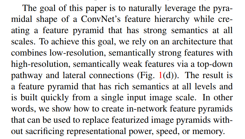
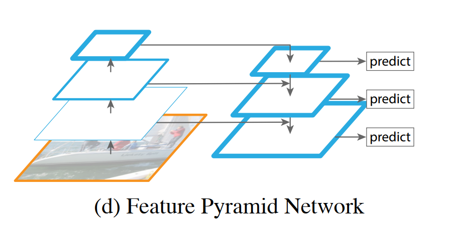
“The goal of this paper is to naturally leverage the pyramidal shape of a ConvNet’s feature hierarchy while creating a feature pyramid that has strong semantics at all scales.”
After meticulously outlining the problem, the authors now state their goal with perfect clarity. They want to take the “free” but flawed pyramid that exists inside a ConvNet and transform it into a new pyramid where every single level is semantically powerful and useful for object recognition.
To do this, they propose an architecture designed to explicitly bridge the semantic gap.
“To achieve this goal, we rely on an architecture that combines low-resolution, semantically strong features with high-resolution, semantically weak features via a top-down pathway and lateral connections (Fig. 1(d)).”
This single sentence is the architectural heart of the entire paper. Let’s define the two key components they introduce:
Top-Down Pathway: This is the process of propagating information from the deepest, most semantically rich layers of the network back down towards the shallower layers. It starts at the top of the pyramid (the small, semantically strong feature map) and progressively upsamples it to increase its spatial resolution. The purpose of this pathway is to carry the high-level semantic information downwards, like a supervisor giving high-level context to their team.
Lateral Connections: These are the merge points. As the top-down pathway brings high-level semantic information to a larger scale, the lateral connection takes the corresponding feature map from the original feedforward pass (the one that is high-resolution but semantically weak) and merges it with the upsampled map. This fusion is the crucial step. It enriches the spatially precise features from the shallower layers with the powerful semantic context from the deeper layers.
“The result is a feature pyramid that has rich semantics at all levels and is built quickly from a single input image scale. In other words, we show how to create in-network feature pyramids that can be used to replace featurized image pyramids without sacrificing representational power, speed, or memory.”
The final result, as shown in Figure 1(d), is a brand new set of feature maps. This new pyramid has the best of both worlds: each level has both strong semantic features and high spatial resolution, making it ideal for detecting objects across a wide range of scales.
Crucially, this entire structure is built inside the network from a single input image. It solves all the problems of the classic featurized image pyramid:
- It’s fast because it requires only one forward pass through the network.
- It’s memory-efficient, allowing the model to be trained end-to-end.
- It has no train-test discrepancy.
The authors are making a bold claim: they have found a way to get the accuracy benefits of a feature pyramid without paying the computational price.
The Fundamental Problem: The core challenge is detecting objects at vastly different scales. A robust detector must be able to find a tiny object in the distance just as well as a large one up close.
The Classic Solution (And Its Failures): The traditional method is the featurized image pyramid.
- How it works: You create scaled copies of the input image and run your feature extractor (e.g., a ConvNet) on each one.
- Its Strength: It achieves “scale invariance,” making it very accurate.
- Its Flaws: This approach is a computational nightmare. It’s incredibly slow for inference, uses too much GPU memory to train end-to-end, and often leads to a mismatch between how the model is trained and how it’s tested.
The “Free” In-Network Pyramid (And Its Flaw): Every standard ConvNet naturally creates a pyramid of feature maps as data flows through it and gets subsampled. This pyramid is computationally free, but it’s deeply flawed due to the semantic gap.
- Semantically Weak Features: Found in the early layers, these feature maps have high spatial resolution (they know where things are) but only represent simple patterns like edges and textures (they don’t know what things are).
- Semantically Strong Features: Found in the deep layers, these feature maps have low spatial resolution but represent high-level concepts (they know what things are, but not precisely where).
Previous Attempts to Bridge the Gap:
- Single-Scale Detectors (e.g., Faster R-CNN): Ignored the problem for speed. They used only one semantically strong, low-resolution map from the end of the network, which compromised accuracy, especially on small objects.
- The Single Shot Detector (SSD): Acknowledged the problem. It made predictions from multiple layers but, to avoid the semantically weak early layers, it discarded them. This decision handicapped its ability to detect small objects.
The FPN’s Proposed Solution: The core idea of this paper is to fix the “free” in-network pyramid.
- The Goal: Create a new feature pyramid where every single level is both semantically strong and has high spatial resolution.
- The Mechanism: An architecture with two key components:
- A top-down pathway to bring the high-level semantic information from the deep layers back up.
- Lateral connections to merge this semantic information with the spatially precise information in the shallower layers.
A Pyramid of Predictions, Not a Single High-Resolution Map
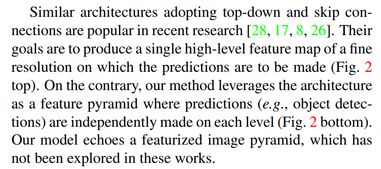
“Similar architectures adopting top-down and skip connections are popular in recent research [28, 17, 8, 26]. Their goals are to produce a single high-level feature map of a fine resolution on which the predictions are to be made (Fig. 2 top).”
The authors are aware that they weren’t the first to use a top-down pathway with skip/lateral connections. This architectural pattern, often called an “encoder-decoder” or “hourglass” structure, is famously used in models like U-Net for biomedical image segmentation and Stacked Hourglass Networks for human pose estimation.
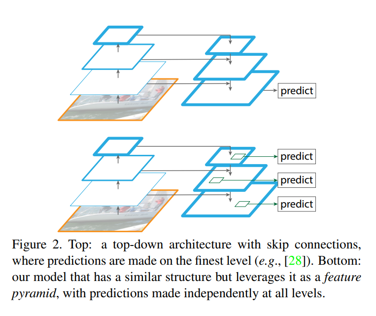
Here’s how those models work, as illustrated in Figure 2 (top) of the paper:
- Encoder (Downsampling Path): They first process the input image through a standard ConvNet, progressively shrinking the feature maps while increasing their semantic depth. This is the “contracting” path.
- Decoder (Upsampling Path): They then take the final, small, semantically strong feature map and progressively upsample it back to the original image resolution.
- Skip Connections: At each upsampling step, they use skip connections to bring in the high-resolution feature maps from the corresponding stage of the encoder. This helps the decoder recover the fine-grained spatial detail that was lost during downsampling.
The crucial point is the end goal: these architectures work to produce one single, final feature map that is both high-resolution and semantically strong. All predictions (e.g., a segmentation mask) are then made based on this final, unified output.
“On the contrary, our method leverages the architecture as a feature pyramid where predictions (e.g., object detections) are independently made on each level (Fig. 2 bottom). Our model echoes a featurized image pyramid, which has not been explored in these works.”
This is where FPN takes a completely different philosophical path. The fundamental difference lies not in the architectural components (top-down path, lateral connections), but in their purpose.
FPN does not aim to create a single, massive, high-resolution output map. Instead, it uses the top-down and lateral connections to create a set of new feature maps at multiple scales. Each of these maps is semantically rich. The key insight is to then make predictions independently on each of these levels.
Think of it like this:
- U-Net Style (Fig. 2 top): Weave one giant, fine-meshed fishing net to catch all fish, big and small. The final net is the only thing you use.
- FPN Style (Fig. 2 bottom): Create a set of specialized nets. Use a large-mesh net to catch big fish (large objects on the low-resolution P5 map), a medium-mesh net for medium fish (medium objects on P4), and a fine-mesh net for small fish (small objects on the high-resolution P3/P2 maps).
By making independent predictions at each level of its new pyramid, FPN is directly mimicking the behavior of the classic (but slow) featurized image pyramid. This is a novel use of the hourglass structure, tailored specifically for the multi-scale nature of object detection.
The FPN Advantage: Claims and Contributions
“We evaluate our method, called a Feature Pyramid Network (FPN), in various systems for detection and segmentation… Without bells and whistles, we report a state-of-the-art single-model result on the challenging COCO detection benchmark [21] simply based on FPN and a basic Faster R-CNN detector [29], surpassing all existing heavily-engineered single-model entries…”
Having established their architectural novelty, the authors now lay out the tangible results. They officially name their architecture the Feature Pyramid Network (FPN) and state that its benefits are not theoretical. When plugged into a standard Faster R-CNN framework, the FPN module alone is powerful enough to achieve state-of-the-art results on the difficult COCO dataset.
The phrase “without bells and whistles” is a statement of confidence. It means their success isn’t due to a complex ensemble of models or dozens of small engineering tricks (like specialized data augmentation or context modeling). The performance gain comes directly from the strength of the FPN architecture itself. They even provide concrete numbers for the improvement over a very strong baseline (Faster R-CNN with a ResNet backbone):
- A massive 8.0 point increase in Average Recall (AR) for the Region Proposal Network (RPN), meaning it’s much better at finding potential objects.
- A significant 2.3 point increase in COCO-style Average Precision (AP) for the final detector, a direct measure of improved detection accuracy.
“In addition, our pyramid structure can be trained end-to-end with all scales and is used consistently at train/test time… Moreover, this improvement is achieved without increasing testing time over the single-scale baseline.”
Finally, the authors circle back to the practical problems they identified at the start of the introduction and explain how FPN solves them. This paragraph highlights the practical genius of their approach:
- End-to-End Training: Unlike classic image pyramids, the FPN is efficient enough to be trained as a single, unified system.
- No Train/Test Discrepancy: Because it can be trained end-to-end, the network sees a multi-scale representation during both training and inference, eliminating this key inconsistency.
- No Speed Penalty: This is perhaps the most impressive claim. FPN delivers the accuracy benefits of a multi-scale pyramid representation without slowing down inference time compared to the standard single-scale baseline detector.
The introduction concludes by framing FPN not just as a new model, but as a fundamental and practical tool that can advance computer vision research.
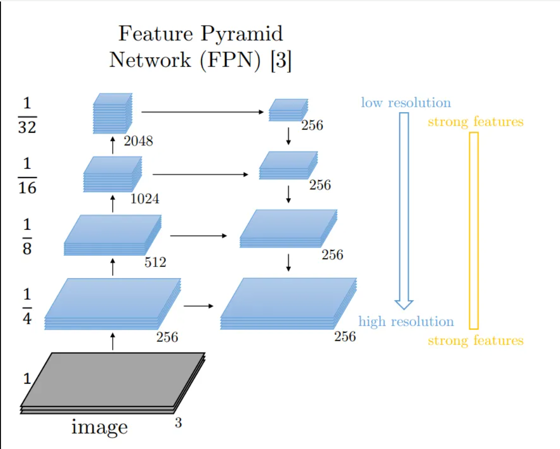
Image source: CloudFactory > Computer Vision model architectures > FPN
2. Related Work
Hand-Engineered Features and Early ConvNets
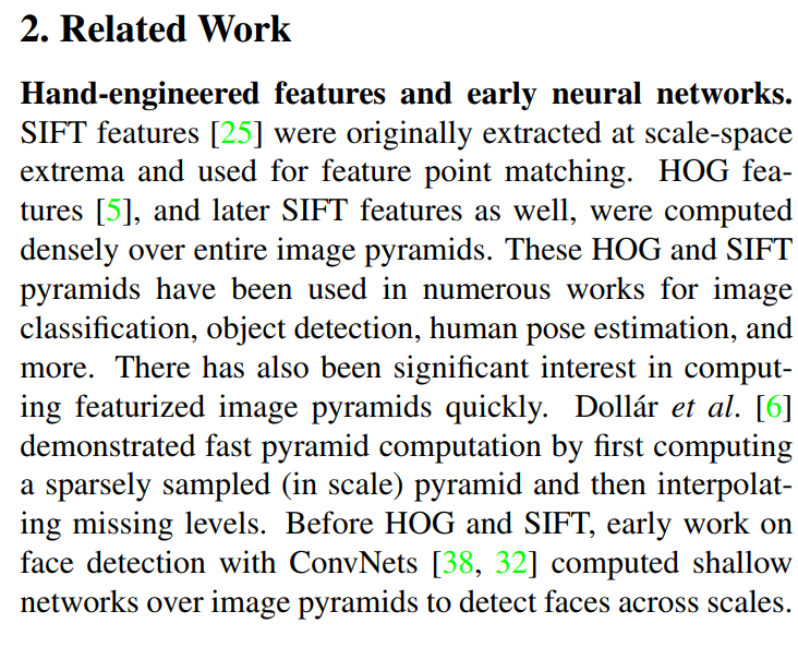
“HOG features [5], and later SIFT features as well, were computed densely over entire image pyramids. These HOG and SIFT pyramids have been used in numerous works for image classification, object detection, human pose estimation, and more.”
This first section provides a historical recap, reinforcing points made in the introduction. Before the dominance of deep learning, progress in computer vision was driven by the design of clever hand-engineered features. SIFT (Scale-Invariant Feature Transform) and HOG (Histograms of Oriented Gradients) were two of the most successful. These algorithms converted image patches into feature vectors that captured essential information about textures and shapes.
However, these features were not inherently robust to large changes in object size. The go-to solution was, once again, the featurized image pyramid. To find objects of all sizes, a detector would analyze HOG or SIFT features computed on every level of an image pyramid. This paradigm was the foundation of state-of-the-art systems for nearly a decade.
“There has also been significant interest in computing featurized image pyramids quickly. Dollár et al. [6] demonstrated fast pyramid computation by first computing a sparsely sampled (in scale) pyramid and then interpolating missing levels.”
The authors make an important point here: the computational cost of image pyramids has always been a problem. Even before the era of massive deep learning models, researchers were looking for shortcuts. They cite the work of Dollár et al., who proposed a clever trick: instead of computing features on, say, 10 different scales, you could compute them on just a few sparse scales (e.g., scale 1, scale 4, scale 8) and then approximate the feature maps for the in-between scales using interpolation. This is an early example of trying to get the benefits of a dense pyramid without paying the full price.
Finally, the authors note that even the first forays into using ConvNets for tasks like face detection followed this same pattern. Early, shallow neural networks were simply used as more powerful feature extractors, but they were still applied in a sliding-window fashion across a multi-scale image pyramid. This shows just how foundational the image pyramid concept has been in the history of object detection.
Deep ConvNet Object Detectors
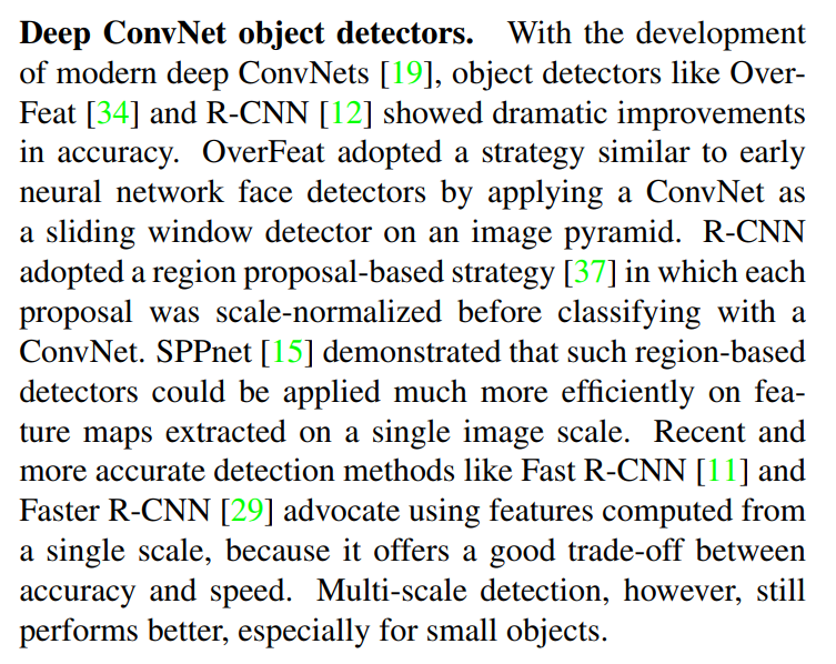
“With the development of modern deep ConvNets [19], object detectors like Over-Feat [34] and R-CNN [12] showed dramatic improvements in accuracy.”
The authors now move into the deep learning era, which began in earnest around 2012. The first wave of deep learning-based object detectors achieved groundbreaking accuracy, but they approached the scale problem in different ways.
OverFeat: This model largely stuck to the classical approach. It used a powerful ConvNet as a feature extractor and ran it as a sliding window detector across a multi-scale image pyramid. It was accurate but inherited the slowness of the image pyramid method.
R-CNN (Regions with CNN features): This was a revolutionary two-stage approach.
- Region Proposals: First, it used a traditional computer vision algorithm (like Selective Search) to propose a few thousand potential object locations (“regions of interest” or RoIs) in the image.
- Classification: Then, it took each of these proposed regions, warped it to a fixed size (e.g., 224x224 pixels) regardless of its original shape or size, and fed it through a ConvNet for classification. This step is what the authors mean by “each proposal was scale-normalized.”
R-CNN was a huge leap in accuracy, but it was incredibly slow, as it had to run the entire ConvNet for each of the ~2000 proposals per image.
“SPPnet [15] demonstrated that such region-based detectors could be applied much more efficiently on feature maps extracted on a single image scale. Recent and more accurate detection methods like Fast R-CNN [11] and Faster R-CNN [29] advocate using features computed from a single scale, because it offers a good trade-off between accuracy and speed.”
The major bottleneck in R-CNN was re-computing features thousands of times. The breakthrough came with SPPnet (Spatial Pyramid Pooling network), an idea refined and popularized by Fast R-CNN. The key insight was simple but powerful: Why run the expensive ConvNet thousands of times? Instead, you can run it just once on the entire input image to produce a single, high-level feature map. Then, for each region proposal, you can simply extract the corresponding patch from that feature map.
This was a massive increase in efficiency and made near-real-time detection possible. Faster R-CNN further refined this by replacing the slow, external region proposal algorithm with a small neural network (the Region Proposal Network or RPN) that shared the main ConvNet’s features, creating a single, unified, end-to-end trainable detector.
However, this incredible speed-up came at a cost. To make it work, these models had to extract all their features from a single feature map, typically the last one from the ConvNet’s backbone (e.g., conv5). This single-scale approach was a pragmatic compromise, trading some of the accuracy of multi-scale methods for a huge gain in speed.
“Multi-scale detection, however, still performs better, especially for small objects.”
The authors conclude this section with their recurring theme. Despite the success and speed of single-scale detectors like Faster R-CNN, the brute-force multi-scale approach (using an image pyramid) still yields higher accuracy. The performance gap is especially noticeable for small objects, which are hard to represent well in a single, low-resolution feature map. This perfectly frames the need for a solution like FPN, which promises the best of both worlds.
Methods Using Multiple Layers
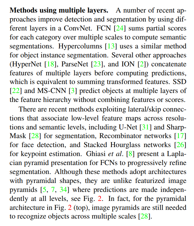
This section can be broken down into two main strategies that other researchers have used to leverage multi-layer features.
Strategy 1: Using the Bottom-Up Pyramid
The authors first discuss methods that use features from the standard, feedforward (bottom-up) feature hierarchy. These approaches fall into two camps:
Combining Features: Models like FCN (Fully Convolutional Networks) for segmentation, Hypercolumns, and ION take features from several different layers (e.g.,
conv3,conv4,conv5), bring them to a common resolution, and then combine them, typically by concatenation or summation. The goal is to create a single, rich feature representation that has both high-level semantics and some low-level detail before making a final prediction. The problem, as always, is that the low-level features are semantically weak.Predicting from Multiple Layers (No Combination): This is the approach taken by SSD (Single Shot Detector) and MS-CNN. They attach prediction heads to multiple layers in the hierarchy and make independent predictions at each level. For example, the head on
conv4is responsible for small objects, and the head on a later layer is responsible for large objects. However, they don’t combine the features between these layers. This means theconv4head is still working with semantically weaker features than the heads on deeper layers.
Strategy 2: Using Top-Down Architectures
“There are recent methods exploiting lateral/skip connections that associate low-level feature maps across resolutions and semantic levels, including U-Net [31] and SharpMask [28] for segmentation…”
The authors then turn to a family of architectures that are structurally the most similar to their own. Models like U-Net and Stacked Hourglass Networks use an encoder-decoder structure with skip connections. They take an image, downsample it to create semantically strong features (the encoder), and then upsample it back to the original resolution, using skip connections to re-inject high-resolution details along the way (the decoder).
This sounds very much like FPN, but the authors draw a critical distinction in their goal.
“Although these methods adopt architectures with pyramidal shapes, they are unlike featurized image pyramids… where predictions are made independently at all levels, see Fig. 2.”
The goal of a U-Net is to produce one single, high-resolution output map that is semantically rich. All predictions are made from this one final result.
FPN uses a similar architecture for a fundamentally different purpose. It does not try to reconstruct a single perfect feature map. Instead, it uses the top-down pathway to create a pyramid of new feature maps (P2, P3, P4, P5), each of which is semantically strong. Then, crucially, it makes independent object predictions on each level of this new pyramid.
This is the key innovation. FPN is the first architecture to use a top-down pathway not to create a single output, but to build a multi-level feature pyramid that can be used just like the classic, featurized image pyramids of the past, but with none of the computational cost. They even note that for the U-Net style models, researchers often still needed to use an image pyramid on top of the model to get the best results, proving that the scale problem wasn’t fully solved.
3. Feature Pyramid Networks
The Core Idea: A General-Purpose Feature Extractor
“Our goal is to leverage a ConvNet’s pyramidal feature hierarchy, which has semantics from low to high levels, and build a feature pyramid with high-level semantics throughout. The resulting Feature Pyramid Network is general-purpose…”
Now we get to the heart of the paper: the architecture itself. The authors begin by restating their clear and ambitious goal: to transform the flawed, “free” pyramid inside a ConvNet into a new, powerful pyramid where every level is rich with semantic meaning.
They immediately emphasize that the FPN is a general-purpose module. This is a crucial point. FPN is not a standalone object detector. Rather, it’s a powerful feature extractor that can be used as a component inside other, more complex systems. Think of it as a turbocharger you can add to an existing detection engine. In this paper, they demonstrate its power by integrating it with the two key components of the Faster R-CNN framework:
- Region Proposal Network (RPN): The part of the detector responsible for identifying potential object locations.
- Fast R-CNN: The part of the detector responsible for classifying those proposed locations.
The Three Key Components
“Our method takes a single-scale image of an arbitrary size as input, and outputs proportionally sized feature maps at multiple levels, in a fully convolutional fashion. This process is independent of the backbone convolutional architectures… The construction of our pyramid involves a bottom-up pathway, a top-down pathway, and lateral connections…”
The authors lay out the blueprint for constructing the FPN. The entire process is fully convolutional, which means it only uses convolutional layers (and no fixed-size fully connected layers). This makes the FPN flexible and allows it to process input images of any size.
Furthermore, the design is backbone-independent. The “backbone” is the main feature-extracting ConvNet (like VGG, Inception, or in this case, ResNet). The FPN module is designed to work with any of these, simply by tapping into the feature maps they produce at different stages.
The construction of the FPN itself consists of three core components, which we will explore in detail next:
- The Bottom-Up Pathway: The standard feedforward pass of the backbone ConvNet, which creates the feature hierarchy with its inherent semantic gap.
- The Top-Down Pathway: The process of upsampling the semantically strong features from the deeper layers.
- Lateral Connections: The crucial links that merge the features from the top-down pathway with the spatially precise features from the bottom-up pathway.
Think of a car’s engine. The main engine block is the backbone. It’s the core component that does the heavy lifting of turning fuel into power. Car manufacturers produce many different engines: small and efficient 4-cylinders, powerful V6s, massive V8s. These are like the different ConvNet backbones: ResNet-50, ResNet-101, VGG16, MobileNet, etc.
Now, imagine you’ve designed a revolutionary new turbocharger. A turbocharger isn’t an engine itself; it’s an add-on module that takes the output of the engine and dramatically boosts its performance.
If you design your turbocharger to only fit a very specific Honda V6 engine, its usefulness is limited. But if you design it as a modular system with standardized connection points, you can adapt it to fit the Honda V6, a Ford V8, or a Toyota 4-cylinder. Your turbocharger is now “engine-independent.”
This is exactly what FPN is. The backbone is the main feature-extracting engine (e.g., ResNet), and the FPN is the high-performance turbocharger that you attach to it.
How FPN Achieves Independence
FPN’s design is clever because it doesn’t need to know the intricate internal details of its backbone. It just needs to be able to “tap into” the backbone’s feature maps at specific points.
Most standard ConvNets are built in stages or blocks. After each stage, the spatial size of the feature maps is halved (e.g., from 56x56 to 28x28).
FPN is designed to connect to the output of these stages. For example, in the ResNet architecture used in the paper:
- The output of the
conv2stage (let’s call itC2) is fed into one of FPN’s lateral connections. - The output of the
conv3stage (C3) is fed into the next lateral connection. - …and so on for
C4andC5.
To use FPN with a different backbone, like MobileNet, you simply identify the corresponding stages in MobileNet where the resolution is halved and connect FPN’s lateral connections to them. The internal logic of FPN (the top-down pathway, the 1x1 convolutions, the element-wise addition) remains exactly the same.
Why This is So Important
Flexibility and Future-Proofing: Researchers are constantly inventing new, better backbones. Because FPN is independent, you can immediately take advantage of these new architectures. When EfficientNet was invented, people could easily combine it with FPN to get an “EfficientDet” model. FPN doesn’t become obsolete when its original backbone does.
Leveraging Pre-training: Backbones are almost always pre-trained on a massive dataset like ImageNet. This teaches them to extract powerful, general-purpose visual features. FPN’s modular design allows you to take a powerful, off-the-shelf, pre-trained backbone and simply bolt the FPN module onto it. You only need to train the small number of layers within the FPN and the final prediction heads, which saves a massive amount of training time and data.
Scalability: It allows you to easily create a family of detectors for different needs.
- Need speed? Use a lightweight backbone like MobileNetV2 + FPN.
- Need accuracy? Use a heavyweight backbone like ResNeXt-101 + FPN.
This “plug-and-play” nature makes FPN an incredibly powerful and versatile tool, not just a single, monolithic model.
The Bottom-Up Pathway: The Backbone’s Forward Pass
“The bottom-up pathway is the feed-forward computation of the backbone ConvNet, which computes a feature hierarchy consisting of feature maps at several scales with a scaling step of 2. … We choose the output of the last layer of each stage as our reference set of feature maps, which we will enrich to create our pyramid.”
The first component, the bottom-up pathway, is the easiest to understand because it’s nothing new. It is simply the standard, feedforward pass of the backbone network (in this case, a ResNet). The term “bottom-up” describes the flow of information from the low-level input pixels (the bottom) to the high-level semantic features (the top).
As the image passes through the backbone, it goes through several stages of computation. A stage is a set of layers that all produce feature maps of the same spatial size. At the end of each stage, a subsampling layer (e.g., a strided convolution) reduces the feature map size, typically by a factor of 2, before the next stage begins.
The authors make a key design decision here. A stage might contain many layers, but for the FPN, they only need one feature map to represent that entire stage. Logically, they choose the output of the final layer in each stage. This makes perfect sense: as information progresses through a stage, its features become more and more abstract and powerful. The final layer’s output, therefore, represents the strongest semantics available at that particular scale.
“Specifically, for ResNets [16] we use the feature activations output by each stage’s last residual block. We denote the output of these last residual blocks as {C2, C3, C4, C5} for conv2, conv3, conv4, and conv5 outputs, and note that they have strides of {4, 8, 16, 32} pixels with respect to the input image.”
Here, the authors provide the concrete implementation details for a ResNet backbone. They designate the outputs of the final residual block of stages 2, 3, 4, and 5 as their reference feature maps. These are labeled C2, C3, C4, and C5, respectively.
The stride is a critical concept. A stride of {4, 8, 16, 32} means:
- Moving 1 pixel in the
C2feature map corresponds to a 4-pixel jump in the original input image. - Moving 1 pixel in the
C5feature map corresponds to a 32-pixel jump in the original input image.
This quantifies the progressive loss of spatial resolution as we go deeper into the network.
“We do not include conv1 into the pyramid due to its large memory footprint.”
This is a crucial and practical engineering decision. The output of the first stage, C1, has a very high spatial resolution (e.g., 112x112 for a 224x224 input) and a huge number of channels. Including it in the pyramid would dramatically increase the GPU memory required, for what is likely a minimal gain in accuracy, since its features are very low-level (simple edge detectors).
So, the bottom-up pathway simply runs the backbone network and saves the output maps from the end of each stage (C2 through C5). These are the raw materials—spatially precise but semantically mismatched—that the rest of the FPN will now transform.
The Top-Down Pathway and Lateral Connections: Building the Bridge
“The top-down pathway hallucinates higher resolution features by upsampling spatially coarser, but semantically stronger, feature maps from higher pyramid levels. These features are then enhanced with features from the bottom-up pathway via lateral connections.”
Here, the authors beautifully describe the process. The goal is to take the semantically rich but low-resolution maps from the top of the pyramid (like C5) and progressively enrich the semantically weak but high-resolution maps from the bottom (like C2, C3). This is achieved through a carefully choreographed dance between the top-down pathway and the lateral connections.
Let’s walk through the process step-by-step, using Figure 3 as our guide.
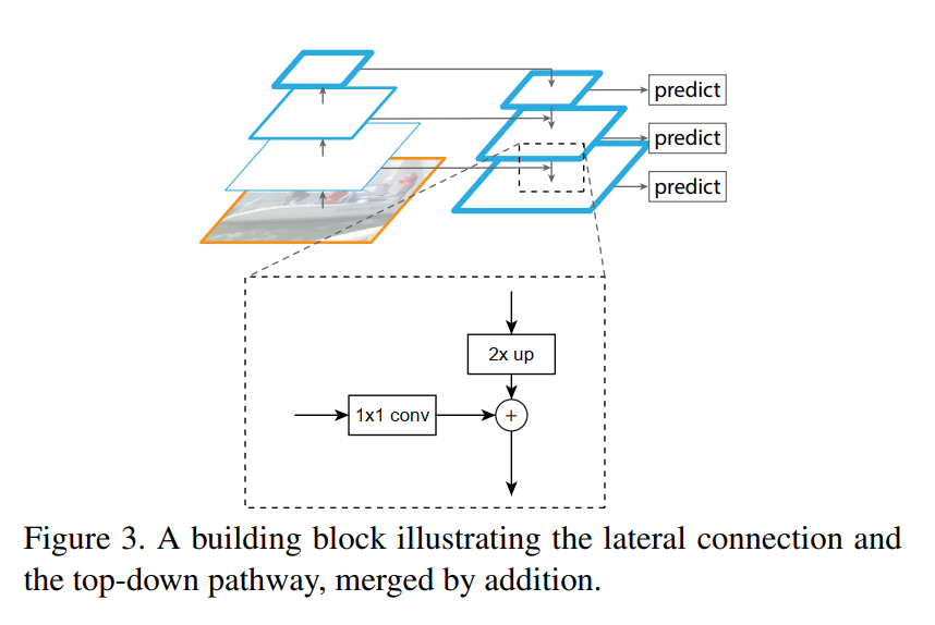
The Step-by-Step Construction
The process is an iteration that starts at the top-most layer (C5) and works its way down.
Initialize the Pyramid: The process begins with the
C5feature map from the bottom-up pathway. This map is already the most semantically powerful. To create the first level of our new pyramid,P5, we simply apply a 1x1 convolution toC5. The main purpose of this is to reduce the number of channels to a fixed, consistent number (the paper uses 256) across all pyramid levels.The Top-Down Step (Upsample): We take the map we just created (
P5) and upsample its spatial dimensions by a factor of 2. For example, ifP5is 14x14, it becomes 28x28. The paper uses simple nearest-neighbor upsampling for this. This upsampled map now contains the strong semantic information fromP5, but spread across a larger area. Its features are powerful but spatially a bit fuzzy.The Lateral Connection (Prepare and Merge):
- Prepare: Now, we reach back to the bottom-up pathway and grab the corresponding feature map,
C4, which also has a 28x28 resolution.C4has precise spatial information but weaker semantics. Before we can merge it, we apply a 1x1 convolution to it. This is a critical step that serves two purposes: it reduces the channel dimension ofC4(which can be very large, e.g., 1024) to match the channel dimension of our upsampled map (256), and it prepares the features for the merge. - Merge: The upsampled map from the top-down path and the prepared map from the lateral connection now have the exact same dimensions (e.g., 28x28x256). The authors merge them using a simple element-wise addition. This is the moment where the semantic information from the deeper layers is fused with the localization information from the shallower layers.
- Prepare: Now, we reach back to the bottom-up pathway and grab the corresponding feature map,
Final Processing: After the addition, a final 3x3 convolution is applied to the merged map. The authors state this is to “reduce the aliasing effect of upsampling.” In simpler terms, this acts like a smoothing step, cleaning up the features after the merge and producing the final, clean feature map for this pyramid level, which we call
P4.Iterate: This process is now repeated. We take our newly created
P4, upsample it by 2x, merge it with a preparedC3, apply a 3x3 convolution, and the result isP3. This continues until the finest-resolution map,P2, is generated.
The final output is a new set of feature maps: {P2, P3, P4, P5}. These maps have the same spatial sizes as the original {C2, C3, C4, C5} maps, but now every single one of them is rich with high-level semantic information. The semantic gap has been bridged.
4. Applications
“Our method is a generic solution for building feature pyramids inside deep ConvNets. In the following we adopt our method in RPN [29] for bounding box proposal generation and in Fast R-CNN [11] for object detection. To demonstrate the simplicity and effectiveness of our method, we make minimal modifications to the original systems… when adapting them to our feature pyramid.”
This opening paragraph sets the stage for the practical part of the paper. The authors reiterate that FPN is a general-purpose, “plug-and-play” module. They will prove its worth by integrating it into the two core components of the Faster R-CNN detector: the Region Proposal Network (RPN) and the Fast R-CNN classifier.
Their emphasis on making “minimal modifications” is important. It signals that FPN is not a complex, sprawling system that requires a complete redesign of the detector. Instead, it’s an elegant drop-in replacement for the standard single-scale feature map, making it easy to adopt.
4.1. Feature Pyramid Networks for RPN
To understand the FPN’s contribution here, we first need a quick refresher on how the original Region Proposal Network (RPN) from Faster R-CNN works.
- Original RPN: The original RPN operates on a single feature map from the backbone (e.g.,
C4). It slides a small network “head” over every location of this map. To detect objects of different sizes, it relies on a set of pre-defined anchors of multiple scales and aspect ratios at each location. In short, it uses multi-scale anchors on a single-scale feature map.
First, let’s set the scene. Imagine you’ve processed an image through a ConvNet and you’re left with a single feature map, let’s say it’s a 38x50 grid of numbers (like C4). Each “pixel” in this grid represents a region of the original image and contains rich semantic information about that region. The problem is: how do you go from this grid of numbers to actual bounding boxes of different sizes and shapes?
This is where anchors come in.
What are “Anchors”?
Think of anchors as a set of pre-defined reference boxes or templates. They are a detector’s “starting guesses” for where objects might be. They are not learned by the network; they are fixed shapes and sizes that you, the designer, choose beforehand.
The paragraph says the RPN uses anchors of “multiple scales and aspect ratios.” This is the key. To detect any object, you need to be prepared for it to be:
- Small, medium, or large (multiple scales)
- Square, tall, or wide (multiple aspect ratios)
So, for every single location on our 38x50 feature map, the RPN places a whole set of these anchor boxes. A typical setup might be 9 anchors per location:
- 3 Scales: A small box, a medium box, a large box.
- 3 Aspect Ratios: A square box (1:1), a tall box (2:1), a wide box (1:2).
(3 scales × 3 aspect ratios = 9 anchors)
At each location on the feature map (yellow dot), the RPN considers a set of anchors with different sizes and shapes.
What is the “Network Head”?
The “head” is a small, separate neural network that “slides” over every location on the feature map. At each location (each of the 38x50 positions), the head looks at the features from the main ConvNet at that spot. Then, for each of the 9 anchors centered at that location, the head makes two predictions:
- “Objectness” Score: It outputs a probability. “How likely is it that this anchor box contains any object vs. just being background?” This is a simple binary classification.
- Bounding Box Regression: It outputs four small correction values (
Δx,Δy,Δw,Δh). “If this anchor does contain an object, how should I slightly move and resize it to fit the object perfectly?” These are the offsets needed to transform the pre-defined anchor into a precise bounding box.
Putting It All Together: “Multi-scale anchors on a single-scale feature map”
This final sentence is the perfect summary. Let’s break it down based on what we’ve learned:
- “a single-scale feature map”: The RPN does all its work on just one feature map (e.g.,
C4). It has no other information about scale from the network itself. - “multi-scale anchors”: To compensate for only having one map, it uses a brute-force strategy. At every single position, it checks for objects of many different potential sizes and shapes using the predefined anchor set.
So, the original RPN’s strategy to handle scale is to stay on one level of the feature hierarchy and use a diverse set of “guess-and-check” boxes to find objects of all sizes. This is clever, but it means the network has to learn to detect both tiny objects and huge objects from the exact same set of features, which is a very difficult task.
The FPN-based RPN fundamentally flips this logic.
“We adapt RPN by replacing the single-scale feature map with our FPN. We attach a head of the same design (3×3 conv and two sibling 1×1 convs) to each level on our feature pyramid.”
Instead of operating on a single map, the new RPN operates on the entire feature pyramid created by FPN: {P2, P3, P4, P5}. A copy of the RPN prediction head is attached to each of these levels. This means the network is now looking for objects at every scale, in a location-dense manner.
“Because the head slides densely over all locations in all pyramid levels, it is not necessary to have multi-scale anchors on a specific level. Instead, we assign anchors of a single scale to each level.”
This is the key simplification and the most elegant part of the design. Since the pyramid itself now handles scale variation, the RPN no longer needs a complex set of multi-scale anchors at every location. The design is changed as follows:
- Anchors of a single scale are assigned to each pyramid level.
- The high-resolution map
P2is responsible for detecting small objects, so it is assigned small anchors (e.g., area of 32² pixels). - The map
P3is assigned larger anchors (64² pixels). - This continues up the pyramid:
P4gets 128² anchors, andP5gets 256² anchors. - Each level still uses anchors of multiple aspect ratios (e.g., tall, wide, square) to handle different object shapes.
“We note that the parameters of the heads are shared across all feature pyramid levels… The good performance of sharing parameters indicates that all levels of our pyramid share similar semantic levels.”
This is a crucial implementation detail. The same prediction head (with the same learned weights) is applied to P2, P3, P4, and P5. This is both parameter-efficient and conceptually powerful. The fact that this works so well is strong evidence for the central claim of the paper: the FPN has successfully created a pyramid where every level has a similarly high semantic strength, allowing a single detector to work effectively across all of them.
In essence, FPN changes the RPN from a detector that uses multi-scale anchors on a single-scale map to a much more effective system that uses single-scale anchors on a multi-scale, semantically rich feature map.
4.2. Feature Pyramid Networks for Fast R-CNN
Once the RPN has proposed a set of candidate bounding boxes (Regions of Interest, or RoIs), the second stage of the detector takes over. This stage, the Fast R-CNN head, is responsible for two things:
- Classifying each RoI (e.g., “this is a car,” “this is a person,” “this is background”).
- Refining the bounding box to fit the object more tightly.
To do this, it needs to extract features for each RoI. In a standard Fast R-CNN, this is simple: you just extract features from the single feature map you’re using. But with FPN, we now have a whole pyramid of feature maps (P2, P3, P4, P5). This presents a new challenge.
The Core Problem: Which Pyramid Level to Use?
An RoI for a tiny car might be 30x40 pixels, while an RoI for a huge bus might be 400x200 pixels. It’s intuitive that we should use a high-resolution feature map (like P2 or P3) to get detailed features for the small car, and a low-resolution map (like P4 or P5) for the large bus. But how do we make this decision in a principled way?
The authors provide a simple and elegant formula to solve this assignment problem.
“We view our feature pyramid as if it were produced from an image pyramid. … Formally, we assign an RoI of width w and height h (on the input image to the network) to the level Pk of our feature pyramid by:
k = ⌊k₀ + log₂(√wh / 224)⌋”
This equation might look intimidating, but it’s actually very intuitive. It’s a formal rule for assigning any given RoI to the most appropriate pyramid level. Let’s break down the anatomy of this equation:
wandhare the width and height of the RoI on the original input image.√whgives us a single number representing the scale of the RoI.224is the canonical ImageNet pre-training size. The authors use this as a reference scale. A 224x224 pixel RoI is considered the “baseline” size.k₀is the target pyramid level for a baseline RoI. The authors setk₀ = 4, which means a 224x224 RoI will be assigned to theP4level.log₂(...)is the magic ingredient. The pyramid levels (P2,P3,P4,P5) have strides that are powers of 2 (4, 8, 16, 32). Thelog₂function perfectly maps the scale of the RoI to this logarithmic structure. If an RoI is half the size of the baseline,log₂(0.5)is -1, meaning it should be assigned to a level one step down (e.g.,k = 4 - 1 = 3). If it’s twice the size,log₂(2)is +1, so it should be assigned one step up (k = 4 + 1 = 5).
An Example in Action
Let’s use the authors’ own intuition. Say we have a smaller RoI that is 112x112 pixels. This is half the baseline size of 224x224. Plugging it into the formula:
k = ⌊4 + log₂(√112*112 / 224)⌋k = ⌊4 + log₂(112 / 224)⌋k = ⌊4 + log₂(0.5)⌋k = ⌊4 + (-1)⌋k = 3
The result is k=3. So, this 112x112 RoI is assigned to the P3 feature map. This is exactly what we want! A smaller RoI is mapped to a finer-resolution feature map (P3 is higher resolution than the baseline P4).
Once an RoI is assigned to a specific pyramid level (e.g., P3), the standard RoI Pooling operation is used to extract a fixed-size feature grid from that map, which is then fed into the final classification and regression heads. This simple formula provides an elegant and effective way to ensure that every object proposal is analyzed at the most appropriate scale.
Imagine you’re a mailroom clerk and you have a set of specialized experts in different rooms.
The Setup
- Your Mail (The RoIs): You have a stack of envelopes. Some are tiny little note cards, some are standard letter-sized envelopes, and some are huge legal-sized packets. These are your RoIs of different sizes.
- Your Experts (The Pyramid Levels): You have a set of experts, each in a different room (
P2,P3,P4,P5).- Expert
P2: Has a magnifying glass. They are brilliant at analyzing tiny details on small note cards but get overwhelmed by large documents. - Expert
P4: Is your generalist. They are perfectly equipped to handle standard, letter-sized envelopes. - Expert
P5: Has a giant desk and thinks in big-picture terms. They are great for summarizing huge legal packets but would miss the details on a tiny note card.
- Expert
The Problem: For every piece of mail that comes in, you need to decide which expert to send it to.
The Formula as a Simple Rulebook
The formula is just the rulebook you, the mailroom clerk, follow. It’s a series of four simple questions:
Question 1: “Is this a standard-sized envelope?” (... / 224)
First, you need a baseline. You decide that a “standard” letter is 224 units wide (just an arbitrary choice, like 8.5x11 inches for paper). You compare every incoming envelope to this standard size. Is it bigger, smaller, or the same? This gives you a ratio.
- A 112-unit envelope is 0.5x the standard size.
- A 448-unit envelope is 2x the standard size.
Question 2: “How many ‘jumps’ in size is it from the standard?” (log₂(...))
Your expert rooms are arranged in a specific way. Each room (P3 vs. P4) is designed for envelopes that are roughly double or half the size of the next. The log₂ part of the formula is just a fancy way of asking: “How many times did I have to double or halve the size to get from my standard envelope to this new one?”
- For the 112-unit envelope (0.5x standard): The answer is -1. (You halved it once).
- For the 224-unit envelope (1x standard): The answer is 0. (No change).
- For the 448-unit envelope (2x standard): The answer is +1. (You doubled it once).
This gives you a “step” count: move -1 rooms, 0 rooms, or +1 rooms.
Question 3: “Where do I start, and where do I end up?” (k₀ + ...)
Your rulebook says that the “standard” mail (the 224-unit envelopes) should always go to your generalist in Room 4. So, k₀ = 4 is your starting point.
Now you just combine the starting point and the number of steps:
- Tiny envelope: Start at Room 4, take -1 step -> Go to Room 3 (
P3). - Standard envelope: Start at Room 4, take 0 steps -> Go to Room 4 (
P4). - Huge envelope: Start at Room 4, take +1 step -> Go to Room 5 (
P5).
Question 4: “What if it’s in between sizes?” (⌊...⌋)
What if you get an envelope that is 1.5x the standard size? The log₂ might give you a weird number like +0.58. Since there’s no “Room 4.58”, the rulebook just says “round down to the nearest whole number.” So you send it to Room 4.
The Big Picture Intuition
The formula is simply a clever and efficient way to map the continuous world of object sizes (a box can be 50 pixels, 51.3 pixels, 1000 pixels…) onto the discrete, logarithmic steps of the feature pyramid. It ensures that every object proposal gets analyzed by the feature map best suited for its scale.
It’s natural to wonder how a specific RoI gets assigned to the right pyramid level. The intuition is exactly as you’d expect: a large RoI (like a bus) should be handled by a low-resolution map (like P5), while a small RoI (like a distant person) is best analyzed by a high-resolution map (like P2).
The crucial detail is how this assignment happens. It’s not a search process. The system doesn’t check the RoI’s size against every pyramid level. Instead, it’s a direct and efficient mapping that works in three simple steps:
Proposals are Defined on the Input Image: The RPN generates proposed bounding boxes with coordinates (
x, y, w, h) that are relative to the original, full-sized image.The Formula is Applied Once: The RoI’s original
widthandheightfrom the input image are plugged into the assignment formula just one time.A Direct Assignment is Made: The formula outputs a single number,
k, which directly points to the correct pyramid level (e.g.,P_k). The RoI is then sent only to that specific level for feature extraction.
Think of it like a mail sorter. The machine reads the zip code (the object’s scale) on the envelope once and sends it directly down the correct chute. It doesn’t have to carry the envelope to every single chute and ask, “Do you belong here?”
In short, the formula acts as a highly efficient routing system, ensuring that every proposed object is instantly matched with the feature map best suited to its scale, without any wasted computation.
5. Experiments on Object Detection
5.1. Region Proposal with RPN
The first test for FPN is to see if it can improve the network’s ability to simply find potential objects. This is the job of the Region Proposal Network (RPN). The key metric here is Average Recall (AR), which essentially asks: “Out of all the real objects in the image, what percentage did our RPN successfully draw a box around?” A higher AR means the RPN is better at finding objects, giving the second stage of the detector better candidates to work with.
Implementation Details
The authors provide standard details for reproducibility, training on the 80-category COCO dataset. They use a ResNet-50 backbone, pre-trained on ImageNet, and train the full RPN with FPN end-to-end.
Ablation Experiments
To prove that their design is effective, the authors perform a series of ablation studies. This is a scientific process where you systematically remove or alter components of your model to see how performance changes. It’s the best way to understand which parts are truly essential. All the results are shown in Table 1 of the paper.
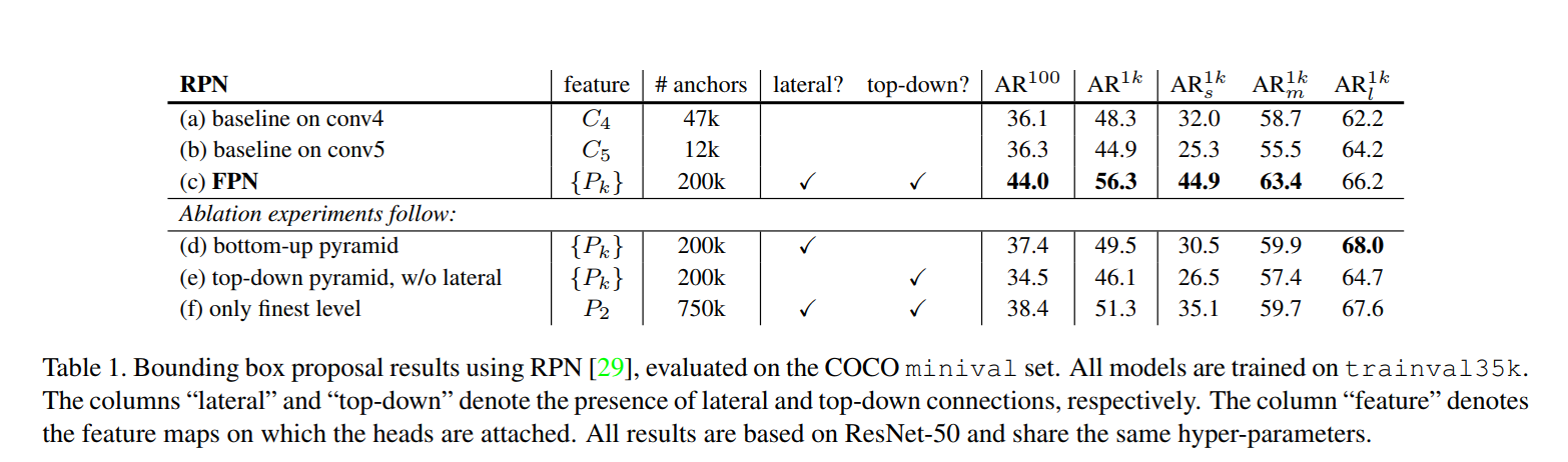
1. Comparison with Baselines
“For fair comparisons with original RPNs [29], we run two baselines (Table 1(a, b)) using the single-scale map of C4 (the same as [16]) or C5… Placing FPN in RPN improves AR¹ᵏ to 56.3 (Table 1 (c)), which is 8.0 points increase over the single-scale RPN baseline (Table 1 (a)). In addition, the performance on small objects (ARs) is boosted by a large margin of 12.9 points.”
- The Baselines (Table 1a, 1b): The authors first establish a baseline using the standard Faster R-CNN approach. Model (a) uses the
C4feature map and gets an AR of 48.3. Model (b) uses the deeper, lower-resolutionC5map, but performance doesn’t improve. This confirms that just using a “stronger” feature map isn’t the answer if you lose too much resolution. - The FPN Result (Table 1c): This is the headline result. By simply replacing the single feature map with their FPN, the AR jumps by 8.0 points to 56.3. This is a massive improvement. Critically, the recall for small objects (
AR_s) skyrockets by nearly 13 points. This is direct evidence that FPN is successfully leveraging high-resolution maps to find the small objects that single-scale detectors typically miss.
2. How Important is the Top-Down Pathway?
“Table 1(d) shows the results of our feature pyramid without the top-down pathway… The results in Table 1(d) are just on par with the RPN baseline… We conjecture that this is because there are large semantic gaps between different levels on the bottom-up pyramid…”
- The Experiment (Table 1d): Here, they test an SSD-style pyramid. They attach prediction heads to the raw
C2, C3, C4, C5maps without any top-down connections to bridge the semantic gap. - The Result: The performance completely collapses, falling right back to the baseline level. This is a critical finding. It proves that simply using features from multiple layers is useless if the early, high-resolution layers are semantically weak. The top-down pathway is essential for enriching these layers with the high-level context needed for object recognition.
3. How Important are the Lateral Connections?
“Table 1(e) shows the ablation results of a top-down feature pyramid without the 1×1 lateral connections… As a results, FPN has an AR¹ᵏ score 10 points higher than Table 1(e).”
- The Experiment (Table 1e): Now they test a pyramid with a top-down pathway (upsampling) but without the lateral connections that merge it with the bottom-up features.
- The Result: Performance is terrible, dropping by 10 points. This shows that the top-down path alone is not enough. While it carries strong semantic information, the repeated process of downsampling and then upsampling has made the feature locations imprecise. Without the lateral connections to re-inject the crisp, well-localized features from the bottom-up pathway, the model knows what is in the image but has lost track of exactly where it is.
4. How Important is Predicting at All Levels?
“Instead of resorting to pyramid representations, one can attach the head to the highest-resolution, strongly semantic feature maps of P2… This variant (Table 1(f)) is better than the baseline but inferior to our approach.”
- The Experiment (Table 1f): Finally, they test whether the pyramid of predictions is truly necessary. They build the full FPN, creating the powerful
{P2, P3, P4, P5}maps, but then only attach the RPN head to the single best feature map,P2. - The Result: Performance is decent (51.3 AR), but significantly worse than the full FPN (56.3 AR). This demonstrates that even with a set of excellent, semantically-strong feature maps, the act of making predictions at multiple scales is still crucial for achieving the best robustness to object size variation.
5.2. Object Detection with Fast/Faster R-CNN
Now that we’ve seen that FPN can generate better object proposals, the next logical question is: can it also improve the final classification of those proposals? To answer this, the authors integrate FPN into the second stage of the detector, the Fast R-CNN head. The main metric here is Average Precision (AP), the standard measure for object detection accuracy in the COCO challenge.
5.2.1. Isolating the Detector: Fast R-CNN on Fixed Proposals
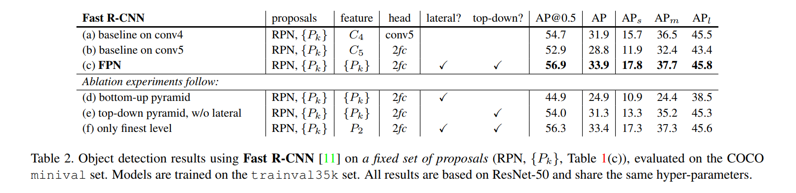
First, the authors conduct another careful ablation study, detailed in Table 2. The goal of this experiment is to isolate the performance of the detector head itself, removing the influence of the RPN. To do this, they generate one high-quality set of proposals using the best FPN-based RPN from the previous section and then use this same fixed set of proposals to train and test several different detector heads.
- The Baselines (Table 2a, 2b): The main baseline is a strong ResNet-based detector which uses the
conv5layers as the classification head on top of theC4feature map. It achieves an AP of 31.9. - The FPN Result (Table 2c): When the FPN-based detector head is used (assigning each RoI to the appropriate pyramid level
P_k), the AP increases by 2.0 points to 33.9. This is a significant gain and shows that FPN provides better features for classification, not just for proposal generation. - Ablation: No Top-Down or Lateral Connections (Table 2d, 2e): Just as with the RPN, removing either the top-down pathway or the lateral connections causes a severe drop in accuracy. This reconfirms that both components are essential. The top-down path provides the necessary semantics, and the lateral path provides the precise localization.
- Ablation: Only the Finest Level (Table 2f): An interesting result occurs here. If they use the full FPN to generate the feature maps but only use the finest level (
P2) for RoI pooling, the result (33.4 AP) is only slightly worse than using all pyramid levels (33.9 AP). The authors argue this is because RoI Pooling itself is a “warping-like operation” that is less sensitive to scale. By resizing every RoI’s feature map to a fixed size (e.g., 7x7), it already handles some scale variation. However, using the full pyramid is still demonstrably better.
5.2.2. The Main Event: End-to-End Faster R-CNN
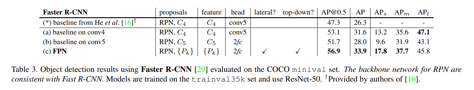
Now for the main result. In this experiment (Table 3), the RPN and Fast R-CNN detector are integrated into a single, end-to-end network that shares the same FPN backbone. This is the true test of the complete system.
- The Baseline (Table 3a): The authors use a very strong single-scale Faster R-CNN baseline with a ResNet-50 backbone, which achieves 31.6 AP.
- The FPN Result (Table 3c): The unified FPN-based Faster R-CNN achieves 33.9 AP. This is a 2.3 point increase in AP and a 3.8 point increase in AP@0.5 (the metric used in the PASCAL VOC challenge). This is a clear and decisive victory for the FPN architecture.
Practical Considerations: Feature Sharing and Running Time
The authors also address two critical real-world factors:
Feature Sharing: When the RPN and Fast R-CNN share the same FPN features, accuracy improves slightly further, and more importantly, inference time is reduced because the features only need to be computed once.
Running Time: This is one of the most compelling results of the paper. The FPN-based Faster R-CNN (running at 0.148 seconds/image) is actually more than twice as fast as the single-scale baseline (0.32 seconds/image). How is this possible? The reason is that the standard ResNet detector uses the entire, very deep
conv5block as its classification head. The FPN architecture, having already incorporated theconv5features into its pyramid, can use a much lighter and faster head (just two small fully-connected layers). This means FPN is not only more accurate but also more efficient.
5.2.3. Taking on the Champions: Comparison with COCO Winners
Finally, the authors pit their best model (using a deeper ResNet-101 backbone) against the top single-model entries from the COCO 2015 and 2016 competitions. As shown in Table 4, the result is stunning.
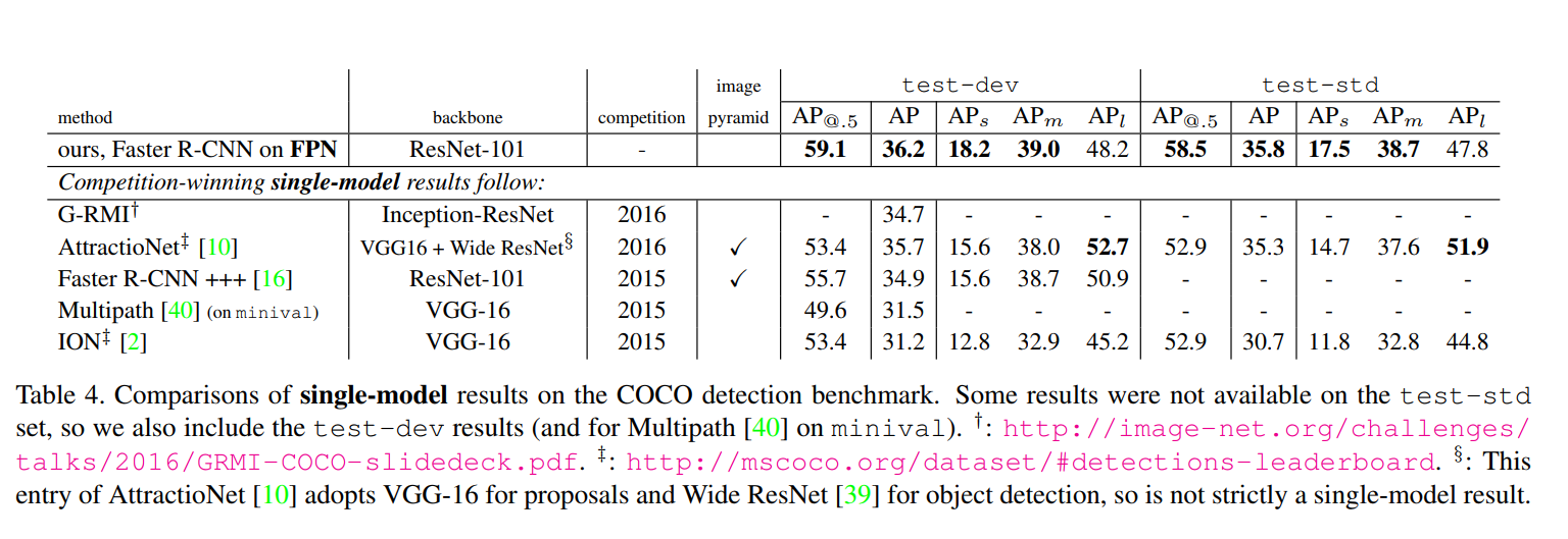
The FPN-based model achieves 36.2 AP on the COCO test-dev set, outperforming the previous state-of-the-art models, including the winners of the COCO challenges. This is the ultimate validation of their approach. It proves that a fundamental architectural improvement can be more powerful than complex, “heavily engineered” systems.
6. Extensions: Segmentation Proposals
Proving FPN’s Generality
“Our method is a generic pyramid representation and can be used in applications other than object detection. In this section we use FPNs to generate segmentation proposals, following the DeepMask/SharpMask framework [27, 28].”
A key claim of the paper is that FPN is a general-purpose tool for any vision task struggling with multi-scale objects. To prove this, the authors extend FPN to the task of instance segmentation proposal generation.
Let’s quickly define that:
- Instance Segmentation: A task that is more challenging than object detection. Instead of just drawing a bounding box around an object, the goal is to produce a pixel-perfect mask that outlines each individual object instance.
- Segmentation Proposals: Similar to the RPN for detection, this is the first stage of a two-stage segmentation pipeline. The goal is not to produce the final, perfect masks, but to generate a large set of high-quality candidate masks that are likely to contain objects.
The previous state-of-the-art methods for this task were DeepMask and SharpMask. These models were powerful but suffered from the exact same problem as classic object detectors: to handle objects of different sizes, they relied on being run on a computationally expensive, multi-scale image pyramid. This makes them a perfect target for demonstrating FPN’s value.
Adapting FPN for Mask Generation
The authors adapt FPN to this new task with a few straightforward modifications, showing the flexibility of their design.
“It is easy to adapt FPN to generate mask proposals. We use a fully convolutional setup for both training and inference. … On top of each level of the feature pyramid, we apply a small 5×5 MLP to predict 14×14 masks and object scores in a fully convolutional fashion, see Fig. 4.”
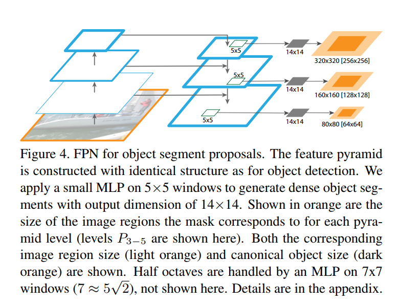
Here’s how the adaptation works:
- Build the FPN: They construct the same FPN as before, creating the set of semantically rich feature maps
{P2, P3, ...}. - Attach a New Head: They replace the RPN’s bounding box prediction head with a new mask prediction head. This head is a small Multi-Layer Perceptron (MLP) implemented as a 5x5 convolution.
- Predict Masks at Each Level: This new head slides over every location of every level of the feature pyramid. At each location, instead of predicting box coordinates, it predicts two things:
- A low-resolution 14x14 mask.
- An “objectness” score, indicating the likelihood that the mask contains an object.
Just as with the RPN, different pyramid levels are responsible for proposing masks for objects of different scales. The high-resolution P2 level will propose masks for small objects, while the low-resolution P5 will propose masks for large objects.
Segmentation Proposal Results
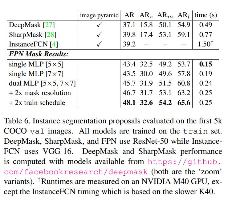
The results, shown in Table 6, are a powerful demonstration of FPN’s effectiveness.
“We also report comparisons to DeepMask [27], SharpMask [28], and InstanceFCN [4], the previous state of the art methods in mask proposal generation. We outperform the accuracy of these approaches by over 8.3 points AR. In particular, we nearly double the accuracy on small objects.”
The FPN-based approach is not just a little better; it’s a massive leap forward.
- Superior Accuracy: The final FPN model achieves an Average Recall (AR) of 48.1, which is 8.3 points higher than the previous best method, SharpMask.
- Dominance on Small Objects: The story is the same as with object detection, but even more dramatic. FPN nearly doubles the recall for small objects (32.6 vs. 17.4 for SharpMask). This is a resounding victory and proves that by properly enriching high-resolution feature maps, FPN can solve one of the most difficult challenges in instance-level recognition.
- Substantially Faster: Because it operates on a single-scale input and avoids building an image pyramid, the FPN-based approach is significantly faster than its predecessors, running at 6-7 FPS.
This section successfully proves the authors’ claim. FPN is not a one-trick pony for object detection. It is a powerful and efficient architectural component that can replace slow image pyramids in a variety of multi-scale vision tasks, leading to models that are simultaneously more accurate and faster.