MobileNetV2 Explained: A Deep Dive into Lightweight Neural Networks

The paper on our reading list is “MobileNetV2: Inverted Residuals and Linear Bottlenecks” by Sandler et al. from Google. This paper is a cornerstone in the world of efficient neural networks, and its ideas are found in countless models running on devices we use every day.
Let’s start where every paper starts: the Abstract.
Diving into the Abstract (Section: Abstract)
The abstract is the paper’s elevator pitch. It’s a super-condensed summary of the problem, the solution, and the results. Let’s unpack it sentence by sentence.
What is MobileNetV2?
In this paper we describe a new mobile architecture, MobileNetV2, that improves the state of the art performance of mobile models on multiple tasks and benchmarks as well as across a spectrum of different model sizes.
Right away, the authors state their main contribution: a new neural network architecture called MobileNetV2. The key takeaways here are:
- “Mobile architecture”: This is designed specifically for resource-constrained devices like smartphones. Think efficiency, low latency, and a small memory footprint.
- “Improves the state of the art”: It’s not just another model; it’s better than the existing mobile models at the time (like its predecessor, MobileNetV1).
- “Multiple tasks”: It’s versatile. The paper will show its effectiveness on more than just image classification.
- “Spectrum of different model sizes”: It’s not a single, fixed-size network. The architecture is scalable, meaning you can tune it to be smaller and faster (with a slight accuracy trade-off) or larger and more accurate, depending on your needs.
More Than Just a Backbone
We also describe efficient ways of applying these mobile models to object detection in a novel framework we call SSDLite. Additionally, we demonstrate how to build mobile semantic segmentation models through a reduced form of DeepLabv3 which we call Mobile DeepLabv3.
This is important. The authors aren’t just presenting a theoretical architecture. They are demonstrating its practical utility. They’ve created specialized, efficient versions of popular models for other common computer vision tasks:
- Object Detection: They introduce SSDLite, a mobile-friendly version of the Single Shot Detector (SSD) framework that uses MobileNetV2 as its backbone.
- Semantic Segmentation: They introduce Mobile DeepLabv3, a lightweight version of the powerful DeepLabv3 model.
This shows that MobileNetV2 is a strong “feature extractor” that can be successfully adapted for complex tasks beyond simple classification.
The Core Contribution: Inverted Residuals and Linear Bottlenecks
This next part is the technical heart of the paper.
Let’s break down these two key phrases:
Inverted Residual Structure: If you’re familiar with ResNet, you know a “residual block” often takes a wide input (many channels), compresses it down to a “bottleneck” (fewer channels), processes it, and then expands it back out to be wide again. The shortcut connection happens between the wide layers. MobileNetV2 flips this on its head, hence “inverted.”
- It starts with a “thin” (low-channel) bottleneck layer.
- It expands it to a much wider layer.
- It processes the features in this wide layer using efficient “depthwise convolutions” (a key ingredient from MobileNetV1). This is where the non-linearity (like a ReLU activation) lives.
- It then projects it back down to a thin bottleneck layer.
- The shortcut connection is between the thin input and thin output bottleneck layers. The structure is thin -> wide -> thin.
Linear Bottlenecks: This is the second crucial insight. The authors claim that applying a non-linear activation function (like ReLU, which kills all negative values) to the thin bottleneck layers is harmful. Why? Because these layers are already low-dimensional. Using ReLU in such a compressed space can easily wipe out valuable information. To prevent this information loss, they simply remove the non-linearity from the bottleneck layers, making them “linear.”
The abstract claims this unique design improves performance and that they’ll provide the intuition behind it.
A Framework for Analysis
Finally, our approach allows decoupling of the input/output domains from the expressiveness of the transformation, which provides a convenient framework for further analysis.
This is a more theoretical point. The “input/output domains” are the thin bottleneck layers, which can be seen as the “capacity” of the block. The “expressiveness of the transformation” is the wide expansion layer, where the complex processing happens. By separating these two, the architecture makes it easier to study and understand their individual roles.
Putting it to the Test
We measure our performance on ImageNet [1] classification, COCO object detection [2], VOC image segmentation [3]. We evaluate the trade-offs between accuracy, and number of operations measured by multiply-adds (MAdd), as well as actual latency, and the number of parameters.
Finally, the authors state how they’ll prove their claims. They use standard, well-respected datasets and, importantly, they don’t just measure accuracy. They evaluate the model on metrics that matter for mobile applications:
- MAdds: A measure of computational cost.
- Latency: The actual time it takes to run on a real device.
- Parameters: The size of the model in memory.
This comprehensive evaluation is key to proving that MobileNetV2 is not just accurate, but genuinely efficient.
1. Introduction
Now that we have the big picture from the abstract, let’s see how the authors frame the problem in more detail in the Introduction. The first couple of paragraphs set the stage for why a model like MobileNetV2 is necessary.
The Big Picture: Accuracy Comes at a Cost (Section 1, Paragraphs 1-2)
This first paragraph paints a familiar picture for anyone in the field of deep learning.
- The Success Story: Neural networks are incredibly powerful. Models like ResNet, VGGNet, and GoogLeNet have achieved amazing, sometimes “superhuman,” results on complex tasks.
- The Catch: This success has a hidden price tag. To get that last bit of accuracy, these state-of-the-art (SOTA) models have become massive and computationally hungry. They require powerful GPUs, lots of RAM, and significant energy to run.
- The Problem: This “cost” makes these giant models completely impractical for on-device applications. You can’t fit a 500MB model that needs a high-end GPU into a smartphone app, a smart camera, or a drone. The resources simply aren’t there.
This establishes the central tension of the paper: the conflict between the quest for accuracy and the constraints of the real world.
The Promise: Breaking the Trade-off
Having laid out the problem, the authors immediately present their solution and its core promise. This paragraph is a masterclass in stating a clear value proposition.
They aren’t just creating another small model. They are aiming for the holy grail of efficient deep learning: reducing computational cost without sacrificing performance.
Let’s look at the key phrase: “…significantly decreasing the number of operations and memory needed while retaining the same accuracy.”
This is the crucial part. It’s relatively easy to make a model smaller and faster if you’re willing to accept a big drop in accuracy (e.g., just remove half the layers). The challenge, and the claim made here, is that MobileNetV2’s architecture is fundamentally smarter. It’s designed to be efficient from the ground up, allowing it to maintain the accuracy of larger models while drastically cutting down on the computational and memory requirements.
In essence, these first two paragraphs tell a simple story:
- Problem: The best AI models are too big and slow for phones.
- Solution: We’ve designed a new architecture, MobileNetV2, that is just as accurate but is small and fast enough to run on your phone.
With the stage set, the paper will now need to deliver the technical details to back up this bold claim. Let’s keep reading.
The Core Idea: The Inverted Residual and Linear Bottleneck Module (Section 1, Paragraph 3)
After setting the stage, the authors waste no time in revealing their secret sauce. This paragraph is the most important one in the introduction, as it explains the novel building block of the entire architecture.
This paragraph succinctly describes the thin -> wide -> thin structure we touched on in the abstract. Let’s visualize the flow of data through this new “module”:
Input: The Bottleneck. The block starts with a “low-dimensional compressed representation.” This means the input tensor has relatively few channels (e.g., 24). This is the “bottleneck.”
Step 1: Expand. The first operation is a 1x1 convolution that expands the number of channels. It takes the thin input and makes it much wider (e.g., expanding from 24 channels to 144 channels). This expansion step creates a high-dimensional space where the model can perform complex transformations.
Step 2: Filter. In this high-dimensional space, the model applies a “lightweight depthwise convolution.” This is the efficient filtering operation inherited from MobileNetV1 that processes each channel independently. This is where the main non-linear transformation (like ReLU6) happens.
Step 3: Project (Linearly). Finally, another 1x1 convolution projects the wide tensor back down to a low-dimensional bottleneck (e.g., from 144 channels back down to 24). The crucial innovation here is that this projection is linear. There is no ReLU or other non-linear activation function applied at the end. This is the “linear bottleneck” part of the name, and it’s designed to prevent information loss in the compressed representation.
The authors also helpfully point out that this is not just a theoretical concept; you can find the code and use it yourself in the TensorFlow-Slim library.
Why This Design is So Good for Mobile (Section 1, Paragraph 4)
The final paragraph of the introduction explains the practical benefits of this specific design, highlighting why it’s more than just an architectural curiosity.
Let’s unpack the two key advantages mentioned here:
1. No Special Operations Needed
The new module is built entirely from standard, highly-optimized deep learning operations (1x1 convolutions, depthwise convolutions, additions). This is a huge practical advantage. It means MobileNetV2 can be implemented easily in any major framework (like TensorFlow or PyTorch) without needing custom code, and it can take full advantage of existing hardware acceleration.
2. The Memory Footprint Advantage
This is a more subtle but incredibly important point for mobile devices. The authors state the module allows them to avoid “fully materializing large intermediate tensors.”
- What does this mean? The “large intermediate tensor” is the wide, expanded layer in the middle of the block. “Materializing” it means fully creating and storing that entire large tensor in memory before moving to the next step.
- The trick: The structure of the inverted residual block is such that deep learning frameworks can be much smarter about memory management. They don’t have to hold that entire huge tensor in memory all at once. They can compute the output in parts, significantly reducing the peak memory usage during inference.
- Why it matters: Mobile and embedded devices have very limited amounts of super-fast cache memory. Accessing the slower main RAM is a major bottleneck that costs time and battery power. By keeping the memory footprint low, the MobileNetV2 block is more likely to fit its computations within the fast cache, leading to significant real-world speedups and power savings.
With the introduction complete, we have a clear understanding of the problem (SOTA models are too big), the proposed solution (a new block with an inverted residual and linear bottleneck structure), and the claimed benefits (high accuracy, low computational cost, and a uniquely low memory footprint).
Next, we will look at the Related Work section to see how this work fits into the broader landscape of deep learning research.
2. Related Work
This section situates MobileNetV2 within the broader field of efficient deep learning. The authors survey the different strategies researchers have used to tackle the fundamental challenge of balancing model accuracy with performance.
The Overarching Goal: The Accuracy/Performance Trade-off
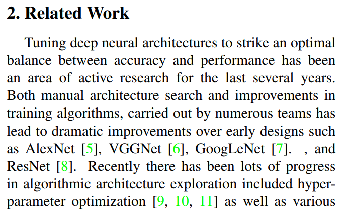
Tuning deep neural architectures to strike an optimal balance between accuracy and performance has been an area of active research for the last several years. Both manual architecture search and improvements in training algorithms, carried out by numerous teams has lead to dramatic improvements over early designs such as AlexNet [5], VGGNet [6], GoogLeNet [7] , and ResNet [8].
The paragraph starts by restating the core problem: finding the “sweet spot” between a model that is smart (accurate) and a model that is fast and small (performant). They acknowledge that early progress was driven by brilliant researchers manually designing iconic architectures like AlexNet and ResNet. These models pushed the boundaries of accuracy but were generally not designed with efficiency as the top priority.
The rest of the paragraph can be broken down into two main philosophies for achieving this balance.
Philosophy 1: Make Big Models Smaller
Recently there has been lots of progress in algorithmic architecture exploration included hyper-parameter optimization [9, 10, 11] as well as various methods of network pruning [12, 13, 14, 15, 16, 17] and connectivity learning [18, 19].
This approach starts with a large, powerful model and then uses algorithms to make it smaller and more efficient. The authors list several techniques:
- Hyper-parameter Optimization: This involves automatically finding the best settings (like learning rates, batch sizes, etc.) to train a model more effectively.
- Network Pruning: This is a very intuitive idea. You train a large, over-parameterized network and then “prune” away the connections or filters that are least important, much like trimming a bonsai tree. The goal is to remove redundancy without hurting accuracy.
- Connectivity Learning: This is a related idea where the model itself learns which connections are important during the training process.
The common thread here is a process of reduction: starting big and algorithmically shrinking down.
Philosophy 2: Design Efficient Building Blocks from the Start
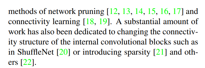
A substantial amount of work has also been dedicated to changing the connectivity structure of the internal convolutional blocks such as in ShuffleNet [20] or introducing sparsity [21] and others [22].
This is a fundamentally different approach. Instead of shrinking a big model, the goal here is to invent new, more efficient building blocks from the ground up. If each block is inherently efficient, the entire network built from these blocks will also be efficient.
The authors specifically call out ShuffleNet [20]. This is a very important reference because ShuffleNet was a direct competitor to MobileNetV2. It introduced clever techniques like pointwise group convolutions and channel shuffling to create a highly efficient architecture.
By mentioning ShuffleNet, the authors are clearly positioning MobileNetV2 in this second camp. They are not presenting a new way to prune ResNet; they are proposing a brand new, fundamentally efficient convolutional block that they believe is superior to other designs like those found in ShuffleNet.
In summary, this paragraph sets up the landscape of efficient network design and places MobileNetV2 squarely in the category of “novel, efficient block design,” setting the stage for a direct comparison with its peers.
Philosophy 3: Let the Machines Do the Designing (Neural Architecture Search)
The authors now introduce a third, more recent, and very powerful approach to finding efficient networks.
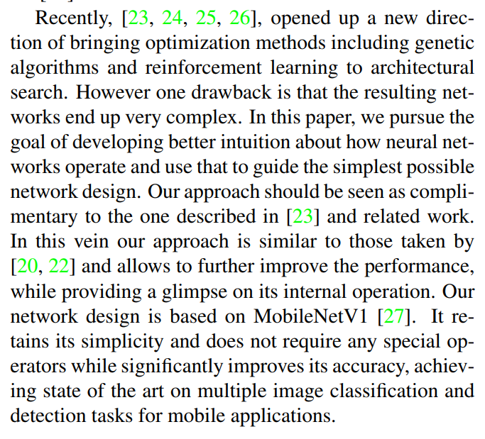
Recently, [23, 24, 25, 26], opened up a new direction of bringing optimization methods including genetic algorithms and reinforcement learning to architectural search. However one drawback is that the resulting networks end up very complex.
This is a reference to the groundbreaking field of Neural Architecture Search (NAS). The idea behind NAS is to automate the design of the neural network itself. Instead of a human researcher trying to invent the best building block, you create an algorithm that searches through millions of possible block designs to find the most optimal one for a given task. The papers referenced ([23] is the famous NASNet paper) use techniques like reinforcement learning to intelligently explore this vast search space.
However, the authors point out a key trade-off. While NAS can produce incredibly high-performing networks (like NASNet), the resulting architectures are often bizarre and counter-intuitive. They can be a complex jumble of different convolutions and connections that work well but are very difficult for a human to understand, analyze, or modify.
MobileNetV2’s Philosophy: Simplicity and Intuition
This is where the authors draw a line in the sand and define their own approach in contrast to NAS.
In this paper, we pursue the goal of developing better intuition about how neural networks operate and use that to guide the simplest possible network design. Our approach should be seen as complimentary to the one described in [23] and related work. In this vein our approach is similar to those taken by [20, 22] and allows to further improve the performance, while providing a glimpse on its internal operation.
This is a powerful statement about their research philosophy.
- Goal: They are not just trying to get a high score on a benchmark. They want to understand the principles of efficient network design. Their goal is to build a model based on clear, simple, and intuitive ideas.
- Positioning: They wisely position their work as “complimentary” to NAS. They aren’t saying NAS is wrong, just that their “human intuition-driven” approach is another valid and valuable path to explore.
- Alignment: They once again align themselves with the creators of models like ShuffleNet [20], who also focused on hand-crafting clever and efficient building blocks.
- Benefit: A key benefit of their approach is interpretability. Because the design is based on simple principles, it provides a “glimpse on its internal operation,” helping the whole research community learn more about what makes these networks tick.
Building on a Strong Foundation
Finally, the authors state the direct lineage of their work.
Our network design is based on MobileNetV1 [27]. It retains its simplicity and does not require any special operators while significantly improves its accuracy, achieving state of the art on multiple image classification and detection tasks for mobile applications.
This is the punchline of the whole section. MobileNetV2 is not a radical departure from everything that came before. It is an evolution of the highly successful MobileNetV1.
They took the core ideas that made MobileNetV1 great:
- Simplicity of the overall architecture.
- Use of depthwise separable convolutions as the core efficient operation.
- No reliance on special operators, making it easy to deploy.
And they improved upon it with their new inverted residual block, leading to a significant boost in accuracy that pushed it to the state-of-the-art for mobile models.
With this context in place, we’re now ready to dive into the technical meat of the paper. The next section, “Preliminaries, discussion and intuition,” will break down the building blocks of MobileNetV2 in detail.
3. Preliminaries, discussion and intuition
Alright, we’re moving into the technical core of the paper. This section lays the groundwork by explaining the key components and the intuition that led to the MobileNetV2 design.
3.1. Depthwise Separable Convolutions
Before we can understand the new contributions of MobileNetV2, we first need to grasp the foundational concept it’s built upon: Depthwise Separable Convolutions. This was the key innovation of its predecessor, MobileNetV1, and it’s still the workhorse here.
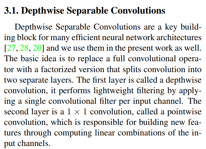
Depthwise Separable Convolutions are a key building block for many efficient neural network architectures [27, 28, 20] and we use them in the present work as well. The basic idea is to replace a full convolutional operator with a factorized version that splits convolution into two separate layers…
To understand why this is so clever, let’s first quickly recap what a standard convolution does.
A standard convolution does two jobs at once:
- It filters the data spatially (e.g., looking for edges or textures in a 3x3 neighborhood).
- It combines features across channels to create new representations (e.g., mixing the information from the red, green, and blue channels to detect the color orange).
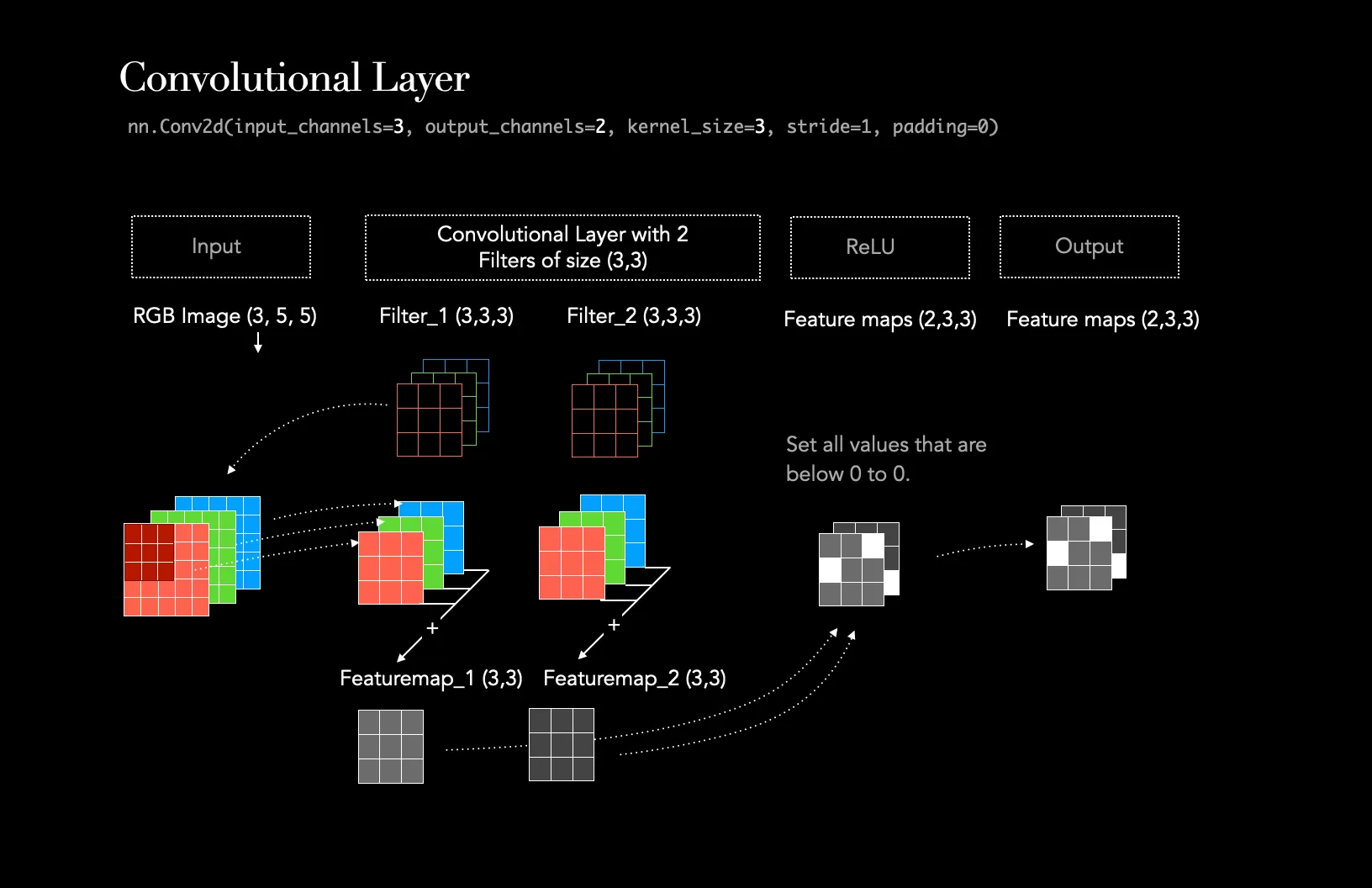
Image taken from Medium post Understanding the Convolutional Filter Operation in CNN’s by Frederik vom Lehn
Doing both of these things at the same time is computationally expensive. The brilliant idea behind Depthwise Separable Convolutions is to “factorize” or split these two jobs into two separate, much cheaper steps.
Step 1: The Depthwise Convolution (Spatial Filtering)
The first layer is called a depthwise convolution, it performs lightweight filtering by applying a single convolutional filter per input channel.
This first step handles only the spatial filtering. Instead of one big, complex filter that works across all channels, you have a set of small, lightweight filters. Crucially, you have exactly one filter for each input channel.
Imagine your input has 3 channels (R, G, B). The depthwise convolution will have:
- One 3x3 filter that slides only over the Red channel.
- One 3x3 filter that slides only over the Green channel.
- One 3x3 filter that slides only over the Blue channel.
At the end of this step, you’ve found spatial patterns (like edges) within each channel independently, but you haven’t mixed any information between the channels yet.
Step 2: The Pointwise Convolution (Channel Mixing)
The second layer is a 1 × 1 convolution, called a pointwise convolution, which is responsible for building new features through computing linear combinations of the input channels.
Now that we have spatially-filtered channels, we need to mix them to create new, meaningful features. This is the job of the pointwise convolution.
A “pointwise” convolution is simply a 1x1 convolution. You can think of it as looking at a single pixel location and performing a weighted sum of all the values across the channels at that one point. This is an incredibly efficient way to compute “linear combinations” of the channels, allowing the network to learn how to best mix the filtered outputs from the depthwise step.
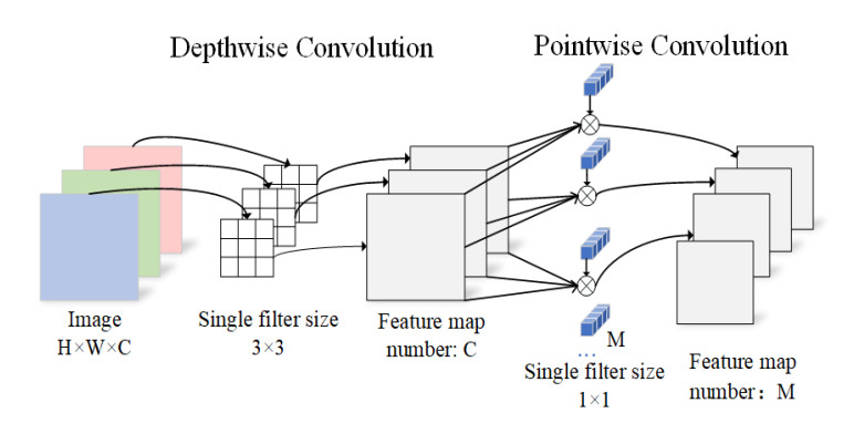
Image taken from paper A lightweight double-channel depthwise separable convolutional neural network for multimodal fusion gait recognition
By splitting the single, expensive standard convolution into two simpler steps—(1) filter each channel spatially, then (2) combine information across channels—we achieve a very similar expressive power with a tiny fraction of the computational cost and parameters. This factorization is the secret behind the efficiency of the entire MobileNet family.
The Math Behind the Magic: Quantifying the Efficiency (Section 3.1, Paragraphs 2-3)
We’ve talked conceptually about how depthwise separable convolutions work, but the real “aha!” moment comes when you look at the numbers. The authors now provide the formulas to prove just how significant the computational savings are.
The Cost of a Standard Convolution
First, let’s establish a baseline. How much does a regular, old-fashioned convolution cost?
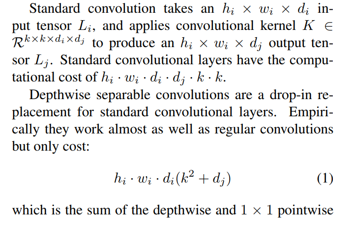
Standard convolution takes an h_i × w_i × d_i input tensor L_i, and applies convolutional kernel K ∈ R^(k×k×d_i×d_j) to produce an h_i × w_i × d_j output tensor L_j. Standard convolutional layers have the computational cost of h_i · w_i · d_i · d_j · k · k.
Let’s decode that formula:
h_i × w_iis the spatial size of the input feature map (height and width).d_iis the number of input channels (the depth).d_jis the number of output channels you want to create.k × kis the size of your convolutional kernel (e.g., 3x3).
The total cost is the product of all these things (h_i · w_i · d_i · d_j · k · k). You can think of it like this: for each of the d_j output channels, you have a big k × k × d_i filter that you slide across all h_i × w_i positions of the input. It’s a massive number of multiplications.
The Cost of a Depthwise Separable Convolution
Now, let’s look at the cost of the more efficient, factorized approach.
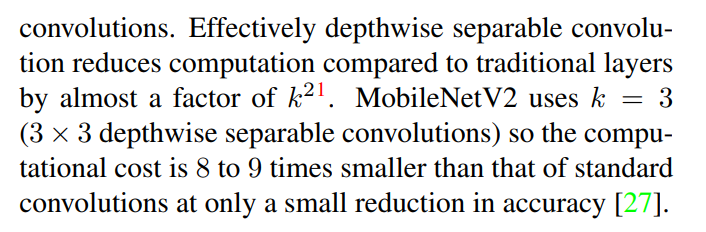
Depthwise separable convolutions are a drop-in replacement for standard convolutional layers. Empirically they work almost as well as regular convolutions but only cost: h_i · w_i · d_i(k² + d_j) (1) which is the sum of the depthwise and 1 × 1 pointwise convolutions.
This formula looks a bit different, but it’s just the sum of the two steps we discussed:
- Depthwise Cost:
h_i · w_i · d_i · k²- This is the cost of sliding
d_idifferentk x kfilters across the input map.
- This is the cost of sliding
- Pointwise Cost:
h_i · w_i · d_i · d_j- This is the cost of the 1x1 convolution that mixes the
d_ichannels to produced_jnew channels.
- This is the cost of the 1x1 convolution that mixes the
When you add them together and factor out the common terms, you get the formula h_i · w_i · d_i(k² + d_j).
The Payoff
Now for the direct comparison. The whole point is that the second formula is dramatically smaller than the first.
Effectively depthwise separable convolution reduces computation compared to traditional layers by almost a factor of k²… MobileNetV2 uses k = 3 (3 × 3 depthwise separable convolutions) so the computational cost is 8 to 9 times smaller than that of standard convolutions at only a small reduction in accuracy [27].
The reduction factor is roughly k². Why? In most deep networks, the number of channels (d_j) is much larger than the kernel size squared (k², e.g., 9 for a 3x3 kernel). So, the cost of the standard convolution (...· d_j · k²) is dominated by multiplying those two large numbers. The separable convolution largely replaces that multiplication with an addition (...· (d_j + k²)), which is much cheaper.
Let’s make this concrete with the paper’s example:
- The most common kernel size is
k=3. - This means
k² = 9. - Therefore, by switching from a standard 3x3 convolution to a depthwise separable 3x3 convolution, you are making the operation roughly 9 times more computationally efficient!
This is an incredible win. The authors note that this massive reduction in cost comes with only a “small reduction in accuracy.” This is the fundamental trade-off that makes MobileNets possible: you sacrifice a tiny bit of model quality for a nearly 9x improvement in computational efficiency. That’s a deal you take every time when designing for mobile devices.
3.2. Linear Bottlenecks
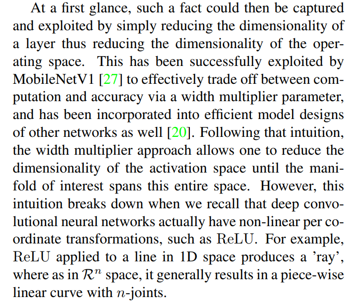
Now we arrive at the second major concept of the paper and the one that is truly novel to MobileNetV2. This section provides the intuition for why the authors made one of their most crucial design choices: removing the non-linearity (ReLU) from the bottleneck layers. The argument is a bit theoretical, but the core idea is fascinating.
The “Manifold of Interest” Hypothesis
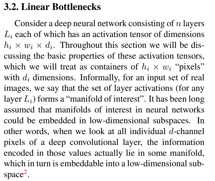
Consider a deep neural network consisting of n layers L_i each of which has an activation tensor of dimensions h_i × w_i × d_i. Throughout this section we will be discussing the basic properties of these activation tensors, which we will treat as containers of h_i × w_i “pixels” with d_i dimensions. Informally, for an input set of real images, we say that the set of layer activations (for any layer L_i) forms a “manifold of interest”.
Let’s break this down.
- An “activation tensor” is just another name for the output feature map of a layer in the network. It is the output of a layer in the network. It’s a big block of numbers with a height, width, and depth (channels).
- The authors ask us to think of this tensor as a collection of
h_i × w_iindividual “pixels”. Each “pixel” is a vector of numbers withd_idimensions (one value for each channel). - Now, imagine you feed your network thousands of real-world images (cats, dogs, cars, etc.). For a specific layer
L_iin the network, you collect all the activation “pixels” that are generated. This huge collection of vectors is what the authors call the “manifold of interest”.
The key insight is that this collection of vectors is not just a random cloud of points in a d_i-dimensional space. It has structure. The activations corresponding to “cat ears” will be different from those for “car wheels,” but they will likely form coherent, lower-dimensional shapes or surfaces within the high-dimensional space. This structured shape is the “manifold.”
The Low-Dimensional Subspace Assumption
The next part is the crucial hypothesis that underpins the entire argument.
It has been long assumed that manifolds of interest in neural networks could be embedded in low-dimensional subspaces. In other words, when we look at all individual d-channel pixels of a deep convolutional layer, the information encoded in those values actually lie in some manifold, which in turn is embeddable into a low-dimensional subspace.
This is the big idea: even though a layer might have, say, 128 channels (d_i=128), the actual information contained in the “manifold of interest” doesn’t actually need all 128 dimensions to be represented. The interesting variations might only exist along, for example, 10 or 20 of those dimensions. The manifold has a lower “intrinsic dimensionality.”
Think of a simple analogy: a long, thin, curved piece of paper (like a ribbon) floating in 3D space.
- The ambient space is 3-dimensional.
- But the paper itself is fundamentally a 2-dimensional surface. You only need two coordinates (length and width) to describe any point on the paper.
- The paper is a 2D manifold embedded in a 3D space.
The authors are arguing that the activation data inside a neural network behaves similarly. The “manifold of interest” (the ribbon) lives inside the high-dimensional activation space (the 3D room), but it can be described and represented in a much lower-dimensional space without losing information.
This assumption is the entire justification for using “bottleneck” layers in networks like ResNet and MobileNet. The purpose of a bottleneck is to project the data into this lower-dimensional subspace, do some processing, and then project it back out. This is efficient because you’re working in a compressed space.
The question that MobileNetV2 tackles next is: what is the wrong way to operate in this compressed, low-dimensional space? And the answer to that will lead us directly to the concept of “linear bottlenecks.”
What is a “Manifold”?
In simple terms, a manifold is a shape that locally looks like simple Euclidean space (like a flat plane), but globally can be curved or twisted.
- Example 1: The Earth’s Surface. Locally, the ground beneath your feet looks flat (2D plane). Globally, the Earth is a sphere (a 2D manifold curved in 3D space).
- Example 2: A Ribbon. A small patch of the ribbon is a flat 2D rectangle. Globally, it can be twisted and curved in 3D space.
The key idea is that a manifold can have a much lower intrinsic dimension than the space it lives in. The Earth’s surface is 2D, but it exists in a 3D world.
Why “of Interest”?
This is the crucial part. The network isn’t interested in every possible combination of pixel values. It’s only interested in the combinations that correspond to real-world things.
Imagine a layer with 128 channels. The total space of all possible activations is a 128-dimensional hypercube. A point chosen randomly from this space would be gibberish—it wouldn’t correspond to any meaningful feature.
However, the activations that are generated when you show the network millions of real images (of cats, dogs, cars, etc.) will not fill this entire 128D hypercube. Instead, they will trace out very specific, structured, lower-dimensional shapes within it.
- There will be a “cat-ear” region of this shape.
- There will be a “car-wheel” region.
- There will be a “blade-of-grass” region.
These regions are all connected and form a complex, curved surface—a manifold. This specific manifold, which represents all the features the network has learned about the real world, is the “manifold of interest”. It’s the only part of the vast activation space that actually matters for the task.
What’s Special About It? (The “Manifold Hypothesis”)
The special thing about the “manifold of interest” is that it’s assumed to be low-dimensional. This is often called the Manifold Hypothesis in machine learning. It’s the assumption that high-dimensional real-world data (like images) actually lies on a much lower-dimensional manifold embedded within that high-dimensional space.
Why is this a reasonable assumption?
Think about all possible 224x224 pixel images. The vast majority of them are just random static noise. The tiny, tiny fraction of images that actually look like something (a face, a tree, a house) all share immense statistical regularities and structure. They are not random. This structure is what confines them to a low-dimensional manifold.
For example, in an image of a face, the position of the left eye pixel is highly correlated with the position of the right eye pixel. They aren’t independent. These constraints and correlations are what reduce the “degrees of freedom” or the “intrinsic dimension” of the data.
This hypothesis is the entire justification for using bottleneck layers, which are designed to compress the feature map down into this low-dimensional “manifold of interest” to perform computations more efficiently.
1. The Mathematical Roots: Differential Geometry
The core term, “manifold,” is a foundational concept from a branch of mathematics called differential geometry. For over a century, mathematicians have used it to study curved spaces (like the surface of a sphere or a donut). The key idea is that even if a shape is globally curved, you can zoom in on any small patch and it looks flat, like a standard Euclidean plane. This allows mathematicians to use the tools of calculus on complex, curved surfaces.
2. The Machine Learning Adoption: “Manifold Learning”
In the late 1990s and early 2000s, machine learning researchers faced a huge problem called the “curse of dimensionality.” Real-world data like images has thousands or millions of dimensions (one for each pixel), making it computationally difficult to work with.
Researchers hypothesized that even though the data lives in a high-dimensional space, the meaningful data points are not randomly scattered. They lie on a much lower-dimensional, smooth, curved surface—a manifold. This became known as the Manifold Hypothesis.
This led to the creation of a whole subfield called Manifold Learning. Famous algorithms like Isomap, Locally Linear Embedding (LLE), and later t-SNE were developed. Their entire purpose was to take high-dimensional data, discover the underlying low-dimensional manifold, and “unroll” it into a flat space, making it easier to visualize and classify.
So, the idea of data lying on a “manifold” became a central concept in machine learning for dimensionality reduction.
3. The Deep Learning Interpretation: Representation Learning
When the deep learning revolution took off, researchers needed a theoretical framework to explain why deep networks were so powerful. They turned to the language of manifold learning.
Pioneers like Yoshua Bengio, Yann LeCun, and Geoffrey Hinton began describing the function of a deep network in geometric terms:
- The input data (e.g., images of faces) lies on a complex, tangled, and twisted manifold. For example, the “face manifold” has variations for identity, pose, lighting, expression, etc.
- The job of each layer in a deep network is to learn a transformation that makes this manifold simpler.
- Layer by layer, the network “untangles” the manifold. It might learn to “straighten out” the variations due to lighting in one layer, and then “flatten” the variations due to pose in another.
- The ultimate goal is to transform the data manifold so that the different classes (e.g., person A vs. person B) become linearly separable—meaning you can separate them with a simple plane.
This geometric view became a very powerful way to understand representation learning.
4. The MobileNetV2 Phrasing: “Manifold of Interest”
The authors of MobileNetV2 are using this well-established language. By adding the phrase “of Interest,” they are being more specific and pragmatic.
They are not talking about some abstract mathematical manifold. They are talking about the specific manifold of feature activations that a network, trained on a specific dataset (like ImageNet), has learned to represent. It is “of interest” because it is the only part of the vast activation space that contains the semantic features (edges, textures, object parts) relevant to the classification task.
Imagine our task is facial recognition. Our input data is a collection of images of two people, Alice and Bob. The network’s job is to learn to separate images of Alice from images of Bob.
The Input: A Tangled Mess of a Manifold
In the raw pixel space, the “face manifold” is a complete mess. It’s a high-dimensional, tangled-up surface where many different factors of variation are all mixed together.
Consider four specific input images:
- Alice_Day.jpg: Alice in bright daylight, looking straight ahead.
- Alice_Night.jpg: Alice in dim lighting, looking straight ahead.
- Bob_Day.jpg: Bob in bright daylight, looking straight ahead.
- Bob_Night.jpg: Bob in dim lighting, looking straight ahead.
If we plot these four points in the high-dimensional pixel space, they might be arranged like this:
Alice_Day <--- (close) ---> Bob_Day
    |                         |
 (far)                    (far)
    |                         |
Alice_Night <---(close) ---> Bob_Night
Notice the problem:
- The distance between
Alice_DayandBob_Dayis small (because the lighting is the same). - The distance between
Alice_DayandAlice_Nightis large (because the lighting is very different).
You cannot draw a simple line (or plane) to separate Alice’s pictures from Bob’s. The manifold is “tangled” by the variation in lighting.
Layer by Layer: The Untangling Process
The job of the deep network is to learn a series of transformations that gradually “untangle” this manifold.
Layer 1: “Straightening out” Lighting Variations
The first few layers of a CNN typically learn to recognize low-level features like edges, gradients, and textures. Let’s say one of these early layers learns a set of filters that are invariant to absolute brightness. These filters might learn to detect the shape of a nose or the curve of an eye, regardless of whether it’s brightly lit or in shadow.
After passing through this layer, the representation of our four points might be transformed. In this new, learned feature space, the points might look like this:
Alice_Day   <---(far)--->   Bob_Day
   |                           |
(close)                     (close)
   |                           |
Alice_Night <---(far)--->   Bob_Night
What happened? The network has learned a transformation that “straightens out” or “flattens” the manifold along the axis of lighting variation. Now, the two images of Alice are close to each other, and the two images of Bob are close to each other. The distance between them is now dominated by the features that define their identity, not the lighting.
However, the manifold might still be tangled by another factor, like pose (head turned left vs. right).
A Later Layer: “Flattening” Pose Variations
A deeper layer in the network might learn more abstract features. For example, it might learn a representation of a “canonical, forward-facing face.” It learns to recognize a nose as a nose, even if it’s seen from the side, and then represents it in a pose-independent way.
After passing through this layer, the transformation might further untangle the manifold. It “flattens” the variations due to pose, so that an image of Alice looking left is now very close to the image of Alice looking right in this new feature space.
The Final Goal: Linear Separability
After passing through many layers, each untangling the manifold along a different axis of variation (lighting, pose, expression, scale, etc.), the final representation of the data becomes very simple.
In the ideal case, all the points corresponding to Alice will be clustered together in one region of the final feature space, and all the points corresponding to Bob will be in another.
Crucially, these two clusters will be linearly separable. This means you can now draw a simple hyperplane (a flat “wall”) between the two clusters to perfectly separate them. This is the job of the final classification layer (e.g., a softmax layer).
So, the phrase “layer by layer, the network untangles the manifold” is a geometric metaphor for the process of representation learning. The network learns to discard irrelevant information (like lighting) and amplify relevant information (like identity) until the data is so well-organized that a simple linear classifier can solve the task.
The Paradox of Non-Linearity: To Be Expressive, a Layer Must Destroy Information
We just established that ReLU can destroy information by collapsing parts of the input. Now, the authors present a deep and paradoxical insight: this information destruction isn’t just a side effect; it’s intrinsically linked to the very source of a deep network’s power.
Let’s carefully unpack this crucial paragraph.
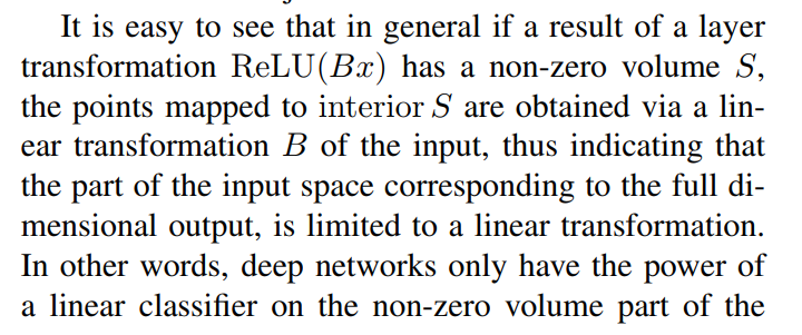
It is easy to see that in general if a result of a layer transformation ReLU(Bx) has a non-zero volume S, the points mapped to interior S are obtained via a linear transformation B of the input, thus indicating that the part of the input space corresponding to the full dimensional output, is limited to a linear transformation. In other words, deep networks only have the power of a linear classifier on the non-zero volume part of the output domain.
This is a dense statement. Let’s translate it into a step-by-step logical argument. The core of the argument revolves around the behavior of the ReLU function.
The Logic Explained:
The Setup: We are looking at a standard layer operation,
ReLU(Bx), wherexis the input feature map andBis a linear transformation (like a convolution or fully-connected layer).The Condition: “Non-Zero Volume”: Let’s assume that the output of this layer isn’t completely squashed into a lower-dimensional shape. It retains its full dimensionality, meaning it has a “non-zero volume.”
The Key Question: What does it take for an output point to be in the “interior” of this output volume?
- The “boundaries” or “edges” of the output shape are created by the
ReLUfunction. Specifically, a boundary is formed whenever one of the output channels is exactly zero. - Therefore, to be in the “interior”—away from all boundaries—an output point
ymust have all of its channels be strictly positive. (y_i > 0for all channelsi).
- The “boundaries” or “edges” of the output shape are created by the
The “Aha!” Moment: What does the
ReLUfunction do to a number that is already positive? Nothing!ReLU(z) = zifz > 0.- This means that for any input
xthat produces an outputyin this “interior” region, theReLUpart of the operation was effectively an identity function. It didn’t do anything at all. - For this part of the data, the transformation was simply
y = Bx.
- This means that for any input
The Staggering Conclusion: The transformation
y = Bxis purely linear. It can only rotate, scale, and stretch the input data. It cannot perform the complex folding, bending, and cutting that gives deep networks their incredible expressive power.
Putting It All Together: The Paradox
The authors have just shown us a profound paradox:
- If a layer preserves the full volume of the input manifold, it can only do so by being a simple linear transformation. It adds no non-linear complexity.
- All the non-linear “magic” of a deep network comes from the
ReLUfunction actively cutting and folding the data manifold. This happens precisely at the boundaries where it sets some channels to zero.
In other words, non-linear power of a deep network—its ability to “fold the paper” into complex shapes—only exists at the boundaries it creates. These boundaries are the “creases” where ReLU is actively setting some channels to zero.
This means:
- Non-Linearity requires information loss. The act of folding the manifold (creating non-linearity) is precisely the act of setting some of its information to zero (collapsing dimensions).
- Preserving information means staying linear. The only parts of the data that pass through the layer with their volume perfectly preserved are the parts that were subjected to a boring, linear transformation.
This explains why simply shrinking a layer (like in MobileNetV1) is so dangerous. A very thin layer has very little room to maneuver. When ReLU starts chopping away at the few dimensions it has, it’s very likely to cause irreparable damage to the “manifold of interest,” leading to a permanent loss of representational power.
This single insight is the entire motivation for the inverted bottleneck structure of MobileNetV2, which we will see is designed to resolve this very paradox.
Imagine a machine learning layer is a magic box that transforms a 2D piece of paper. The box has two internal stages:
Stage B (The Stretcher): This is the linear part,
Bx. It’s like a machine that can stretch, rotate, or skew the paper, but it always keeps straight lines straight. It cannot bend or fold the paper. This is a linear transformation.Stage ReLU (The Folder): This is the non-linear part. This machine takes the paper from Stage B and does one simple, brutal thing: it folds the paper along the x-axis and y-axis. Any part of the paper that is in the bottom half (negative y) gets folded up onto the x-axis. Any part in the left half (negative x) gets folded over onto the y-axis. The entire 2nd, 3rd, and 4th quadrants are squashed onto the positive axes.
The entire layer is the combination: ReLU(Bx).
Now, Let’s Analyze the Output
The output of our magic box will be a shape that only exists in the top-right (first) quadrant. Let’s call this output shape S.
The paper makes a simple claim: “if a result… has a non-zero volume S…” * In our 2D analogy, “volume” just means “area.” So, this means our output shape S isn’t just a line or a point; it’s a real 2D shape that covers some area in the top-right quadrant.
Now for the crucial part: “…the points mapped to interior S…”
What is the “interior” of our output shape S?
- The edges (or boundaries) of
Sare the parts that lie on the x-axis or the y-axis. These are the places where theReLUfolder did its work. - The “interior” of
Sis the part that is NOT on the edges. It’s the fleshy middle part of the shape, where every point has an x-coordinate> 0and a y-coordinate> 0.
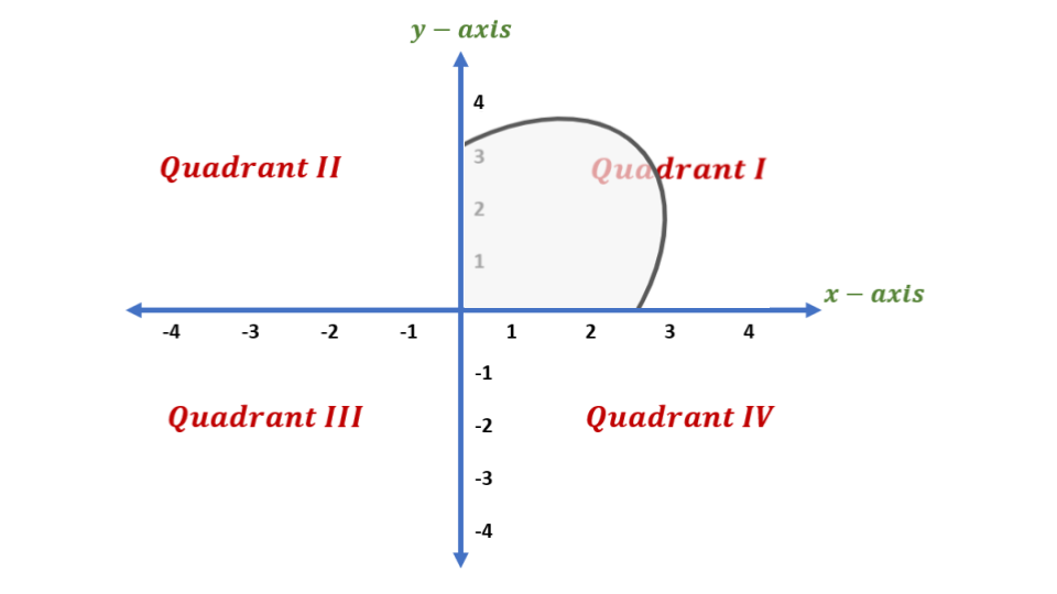
The “Aha!” Moment: What did ReLU do to the interior points?
Let’s pick a single point p_out from the interior of our final shape S. We know for a fact that both of its coordinates are positive.
Now, let’s trace it backward through the ReLU folder. The ReLU folder takes an input p_mid and produces our output p_out.
- Since
p_out’s x-coordinate is positive, theReLUfunction didn’t change it. So,p_mid’s x-coordinate must be the same. - Since
p_out’s y-coordinate is positive, theReLUfunction didn’t change it. So,p_mid’s y-coordinate must be the same.
Conclusion: For any point that ends up in the interior of the final shape, the ReLU folding stage did absolutely nothing! It was a complete pass-through.
So, for this specific subset of the data, the entire transformation was just the work of the first stage, the B stretcher. The transformation was p_out = B * p_in. And we already know that B is a purely linear transformation.
The Punchline (Translating back to the paper)
This is the entire argument:
- A deep network layer gets its power from non-linearity (the
ReLUfolder). - This non-linearity works by collapsing data onto the axes (information loss).
- Any part of the data that survives this collapse with its dimensionality intact (the “interior” with “non-zero volume”) is, by definition, the part that the
ReLUfolder didn’t touch. - Therefore, the transformation for this “surviving” part of the data was purely linear.
In other words: The parts of a network layer that are non-linear are precisely the parts that are destroying information. The parts that preserve information are forced to be linear.
This is why the authors conclude that in a low-dimensional bottleneck, where you can’t afford to lose any information, you must get rid of the ReLU and make the layer purely linear. You must remove the “folder” to protect your precious, un-squashed paper.
A Visual Guide to Linear vs. Non-Linear Transformations with ReLU
In the above post, you’ll find a Python visualization that shows how a ReLU activation function transforms a 2D shape, demonstrating the geometric difference between linear and non-linear operations in a neural network.
The Solution: Using High Dimensions as a Safety Net
So, we’re faced with a paradox: for a layer to be non-linear and powerful, it must use ReLU to cut and fold the data, which risks destroying the “manifold of interest.” But if it avoids this destruction, it remains linear and adds no expressive power. How can we get the best of both worlds? The authors provide the answer in this paragraph.
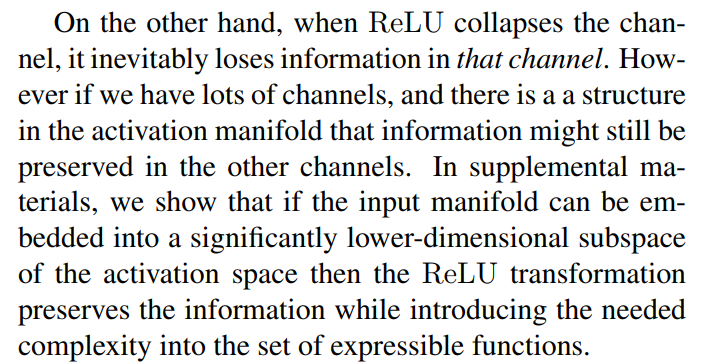
Information is Redundant
First, a simple but important observation:
On the other hand, when ReLU collapses the channel, it inevitably loses information in that channel. However if we have lots of channels, and there is a structure in the activation manifold that information might still be preserved in the other channels.
Think about a color photograph. It has three channels: Red, Green, and Blue. If you were to completely delete the Blue channel, you would lose all the “blue” information. However, you could still easily recognize the objects in the picture. Why? Because the structural information—the edges, shapes, and textures that define a “cat” or a “car”—is highly redundant and is also present in the Red and Green channels.
The authors are arguing that the “manifold of interest” inside a network behaves similarly. The crucial information is often encoded redundantly across multiple channels. So, even if ReLU zeroes out a few channels, the core information can survive in the channels that remain.
The Crucial Condition for Survival
This information survival isn’t guaranteed. It only works under a very specific condition, which is the key insight of this entire section:
In supplemental materials, we show that if the input manifold can be embedded into a significantly lower-dimensional subspace of the activation space then the ReLU transformation preserves the information while introducing the needed complexity into the set of expressible functions.
This is the punchline. Let’s translate it with an analogy.
The Sculpture Analogy:
- Imagine our precious “manifold of interest” is a complex 3D sculpture.
- The “activation space” is the room the sculpture is in.
- The
ReLUoperation is like a destructive process that flattens the room along one dimension, like shining a powerful light from one direction to cast a 2D shadow.
Now, consider two scenarios:
Scenario 1: The Bottleneck (Low-Dimensional Space)
- You place your 3D sculpture in a tiny 3D room. The sculpture nearly fills the entire room.
- Now, you apply the
ReLUprocess and flatten the room into a 2D shadow. - The result? You’ve completely lost one dimension of your sculpture. Its intricate 3D structure is irreparably damaged. You cannot reconstruct the sculpture from its shadow.
- This is what happens when you apply
ReLUin a low-dimensional bottleneck layer. The manifold fills the space, so any information loss is catastrophic.
Scenario 2: The Expansion (High-Dimensional Space)
- Now, you take your same 3D sculpture and place it in a massive 100-dimensional room. Our 3D manifold is now embedded in a significantly higher-dimensional space.
- You apply the
ReLUprocess and flatten the room along one of its 100 dimensions, projecting it into a 99-dimensional “shadow.” - The result? The 3D structure of the sculpture is almost perfectly preserved! Losing one dimension out of 100 is insignificant. The core relationships and shape of the sculpture remain intact in the other 99 available dimensions.
This is the brilliant insight! The way to safely apply the information-destroying ReLU is to first give your manifold plenty of extra dimensions to live in.
By projecting the data into a high-dimensional space (the “expansion” layer in MobileNetV2), you create a safety net. In this expanded space, ReLU can do its job of cutting and folding (introducing non-linearity) by zeroing out some channels, but the risk of destroying the core structure of the “manifold of interest” is dramatically reduced because the information is safely preserved in the many other dimensions that remain.
The Two Guiding Principles of MobileNetV2
After that deep dive into the geometry of information flow, the authors neatly summarize their entire argument into two core principles. These two statements are the “theses” of the paper and the direct justification for their design.
To summarize, we have highlighted two properties that are indicative of the requirement that the manifold of interest should lie in a low-dimensional subspace of the higher-dimensional activation space:
Principle 1: The Expressiveness vs. Information Destruction Trade-off
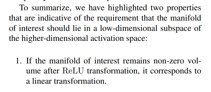
1. If the manifold of interest remains non-zero volume after ReLU transformation, it corresponds to a linear transformation.
This is a restatement of the paradox we discussed. A layer can either be a simple, information-preserving linear transformation, OR it can be a complex, information-destroying non-linear one. You can’t have both at the same time. The only way to get expressive power is to accept that ReLU will collapse parts of the input.
Principle 2: The High-Dimensional Safety Net
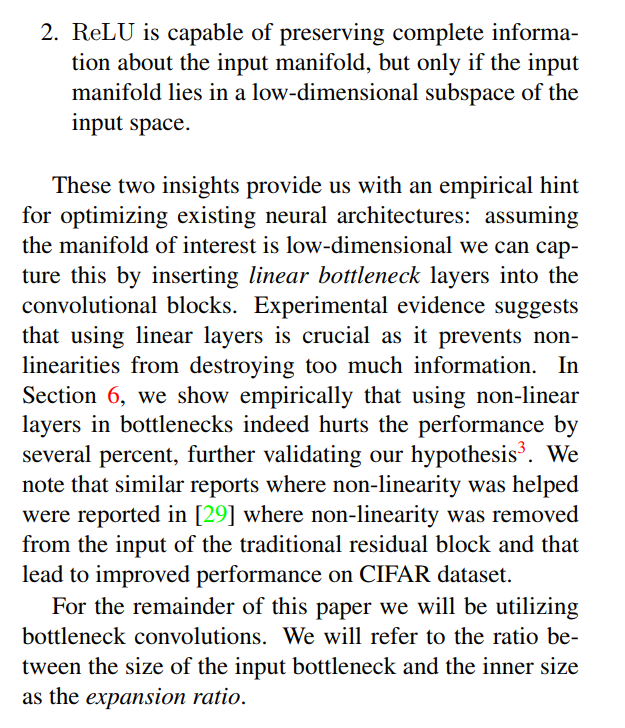
2. ReLU is capable of preserving complete information about the input manifold, but only if the input manifold lies in a low-dimensional subspace of the input space.
This is the solution to the paradox. We can safely let ReLU do its destructive work if and only if we first give our data a high-dimensional “safety net.” By projecting our low-dimensional manifold into a much higher-dimensional space, we ensure that even when ReLU collapses a few of those dimensions, the overall structure of our manifold remains intact in the many dimensions that are left over.
The Design Prescription: Linear Bottlenecks
These two principles don’t just form a neat theory; they give the authors a clear, empirical “hint” for how to design a better network.
These two insights provide us with an empirical hint for optimizing existing neural architectures: assuming the manifold of interest is low-dimensional we can capture this by inserting linear bottleneck layers into the convolutional blocks.
This is the big reveal. The argument flows perfectly:
- We know the important information (the manifold of interest) is low-dimensional.
- Therefore, it makes sense to represent it in a low-dimensional “bottleneck” layer to be efficient.
- BUT, we also know that applying a non-linearity like
ReLUin this confined, low-dimensional space is extremely dangerous and risks destroying the manifold. - THEREFORE, the logical conclusion is to make the bottleneck layers linear. We simply remove the
ReLUfrom the bottleneck to protect our manifold from destruction.
This is the birth of the “Linear Bottleneck.”
Experimental evidence suggests that using linear layers is crucial as it prevents non-linearities from destroying too much information. In Section 6, we show empirically that using non-linear layers in bottlenecks indeed hurts the performance by several percent, further validating our hypothesis³.
The authors don’t just want us to take their word for it. They promise to prove it with experiments. Later in the paper, they will run an ablation study where they add ReLU back into the bottlenecks and show that, as their theory predicts, the model’s performance gets significantly worse.
The Expansion Ratio
Finally, they give a name to the key parameter of their new block design.
For the remainder of this paper we will be utilizing bottleneck convolutions. We will refer to the ratio between the size of the input bottleneck and the inner size as the expansion ratio.
This is a simple but important definition. If a block takes a 16-channel bottleneck as input and expands it to a 96-channel intermediate layer before projecting it back down, the expansion ratio is 6 (96 / 16 = 6). This ratio will be a key hyperparameter for controlling the trade-off between the model’s capacity and its computational cost.
And with that, the theoretical foundation is complete. We now understand the why behind MobileNetV2’s design. The rest of the paper will focus on the what and the how: detailing the exact architecture and proving its effectiveness.
Visualizing the Theory: The Spiral Experiment (Figure 1)
After all that dense theory, the authors provide a simple yet brilliant visualization in Figure 1 to help us build a concrete intuition for their main point: to safely apply ReLU, you must first expand your data into a higher dimension.
Let’s break down what this figure is showing.
The Experiment Setup
The experiment is designed to simulate what happens to a “manifold of interest” inside a network layer.
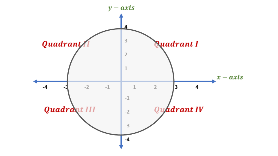
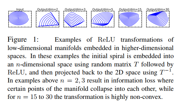
- The Manifold: The input is a simple 2D spiral. This is our toy “manifold of interest.” It’s a 1-dimensional line living in a 2D space.
- The “Expansion”: The spiral is projected from its 2D space into a higher,
n-dimensional space using a random transformation matrixT. This simulates the “expansion” part of the MobileNetV2 block. - The Non-Linearity: The
ReLUfunction is applied to the data in thisn-dimensional space. This is the critical, potentially destructive step. - The “Projection”: Finally, the data is projected back to the original 2D space using the inverse transformation
T⁻¹so we can see what happened to it.
The experiment is repeated for different values of n, the dimension of the intermediate “expansion” space.
Interpreting the Results
The results clearly show two distinct regimes:
Case 1: Low-Dimensional Expansion (n = 2, 3)
- What we see: When the expansion dimension
nis very low (close to the manifold’s own dimension), the output is a disaster. The beautiful spiral structure is completely destroyed. Large segments of the spiral are “collapsed into each other,” squashed onto straight lines. - What it means: This is a visual confirmation of the theory. In a low-dimensional space,
ReLUdoesn’t have enough room to work without causing catastrophic information loss. It’s like our sculpture-in-a-tiny-room analogy; flattening the room destroys the sculpture. The transformation is not invertible; you could never get the original spiral back from these mangled outputs.
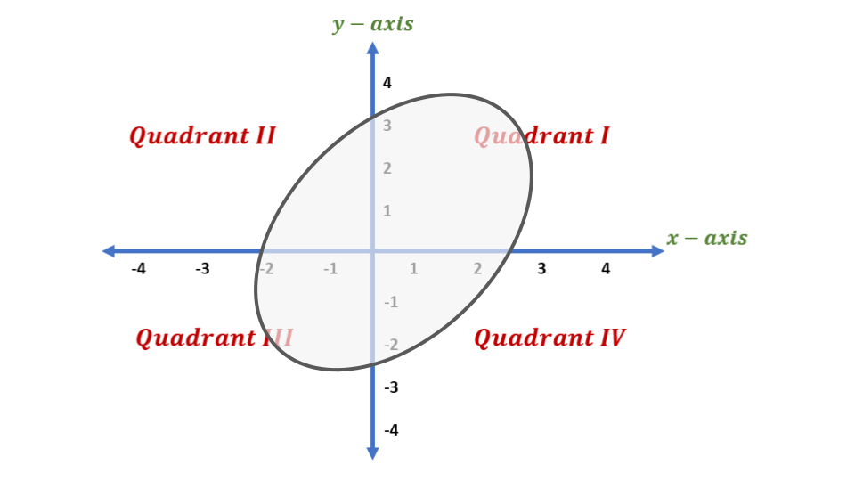
Case 2: High-Dimensional Expansion (n = 15, 30)
- What we see: As we increase the expansion dimension
n, something amazing happens. The output spiral looks almost identical to the input! The information is almost perfectly preserved. - A Subtle, Important Difference: Although the shape is preserved, the transformation is now “highly non-convex.” This means that the
ReLUhas successfully introduced complex, non-linear folds and bends into the space, but it has done so without destroying the underlying structure of the manifold. - What it means: This is the “safety net” in action. By embedding the 2D spiral into a high-dimensional space (like 15D or 30D), we give
ReLUthe freedom to perform its non-linear magic without risking the integrity of our manifold. It’s our sculpture-in-a-huge-room analogy; flattening one dimension out of 30 doesn’t harm the 2D shape of the spiral. The transformation is complex, but it’s also invertible.
This simple figure perfectly illustrates the core design principle of MobileNetV2: the expand -> project structure, where non-linearities are only applied in the high-dimensional expanded space, is the key to creating a powerful and information-preserving building block.
Visualizing MobileNetV2: A Hands-On Guide to Why Linear Bottlenecks Work
In the above postm, I recreate the spiral experiment from the MobileNetV2 paper to visually prove how neural networks can avoid information loss.
The Evolution of an Idea: From Standard Convolution to the Inverted Residual (Figure 2)
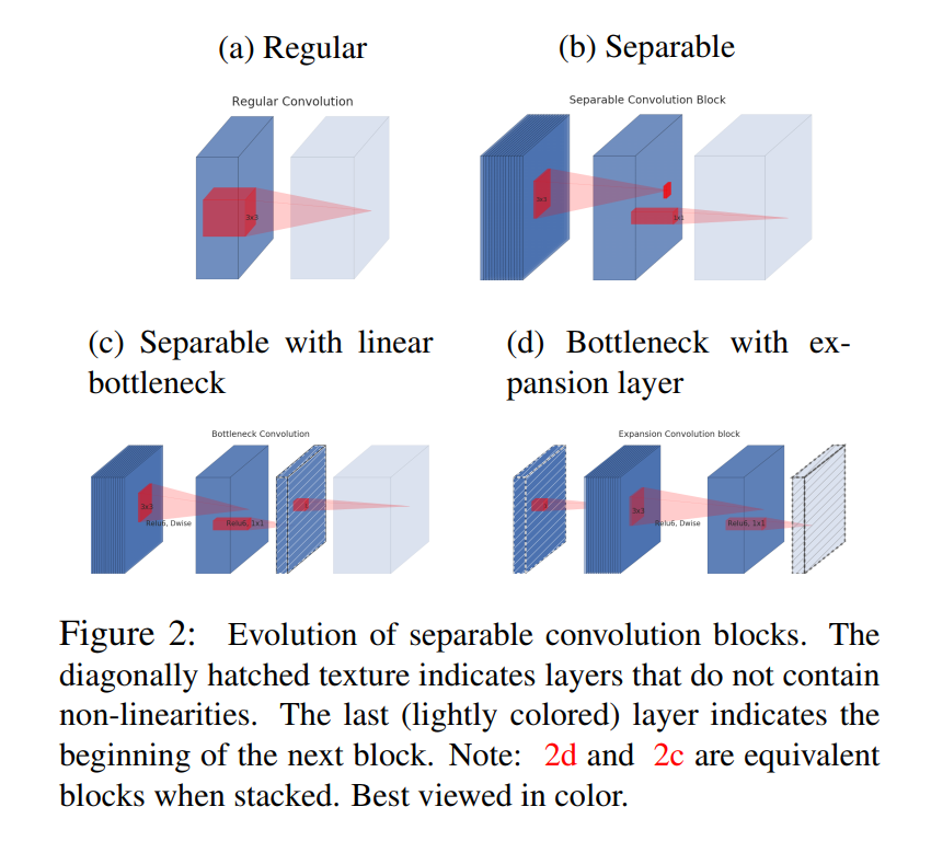
Figure 2 provides a “visual history” of the concepts we’ve covered, showing how each idea builds upon the last, culminating in the final MobileNetV2 block design. The key to understanding this figure is the legend: “The diagonally hatched texture indicates layers that do not contain non-linearities.”
Let’s walk through the evolution step-by-step.
(a) Regular Convolution
- What it is: This is the baseline, the standard, expensive convolution we discussed in Section 3.1. It takes a “wide” input tensor (many channels, represented by the block’s thickness) and produces another wide output tensor.
- How it works: A single, large
3x3kernel (the red cube) operates on both spatial dimensions and channel depth simultaneously. This is computationally costly. - Key takeaway: This is the inefficient operation we want to replace.
(b) Separable Convolution Block
- What it is: This is the core idea from MobileNetV1. It replaces the single expensive convolution with the two-step, factorized version.
- How it works:
- A
3x3Depthwise convolution filters the wide input spatially (one filter per channel). - A
1x1Pointwise convolution mixes the channels to produce the final wide output.
- A
- Key takeaway: This block performs a similar function to (a) but is ~9x more efficient. This is the
wide -> widedesign of MobileNetV1.
(c) Separable with Linear Bottleneck
- What it is: This is the first step towards the MobileNetV2 design, introducing the idea of bottlenecks. This is a
wide -> narrow -> widestructure, similar to a traditional ResNet bottleneck block. - How it works:
- A
1x1convolution projects the wide input down to a narrow “bottleneck” tensor. - A
3x3Depthwise convolution filters this narrow tensor. - A
1x1convolution expands the result back to a wide output.
- A
- The Crucial Detail: Look at the output of the final
1x1expansion. The block is hatched, indicating it is linear. The non-linearity has been removed from this layer to preserve information, as motivated by our theoretical discussion.
(d) Bottleneck with Expansion Layer (The MobileNetV2 Block)
What it is: This is the final, brilliant inversion of the block in (c). Instead of
wide -> narrow -> wide, this is anarrow -> wide -> narrowblock. This is the inverted residual block.How it works:
- It starts with a narrow bottleneck input.
- A
1x1convolution expands it to a much wider intermediate tensor. This creates the “high-dimensional safety net” where ReLU can operate safely. - The
3x3Depthwise convolution filters this wide tensor. This is where the non-linearity is applied. - A final
1x1convolution projects the wide tensor back down to a narrow output bottleneck.
The Crucial Detail: Again, look at the final output layer. The block is hatched. This is the linear bottleneck. The authors have moved the non-linearity inside the block (into the wide expansion part) and kept the final projection linear to protect the low-dimensional output from information loss.
The note that “(2d) and (2c) are equivalent blocks when stacked” is a subtle but important point. If you were to stack multiple blocks of type (c), the linear expansion of one block would feed directly into the projection of the next. The authors found that restructuring it into the narrow -> wide -> narrow form of (d) and using shortcuts between the narrow ends (as we’ll see next) was more memory-efficient and performed slightly better. This is the final, optimized design.
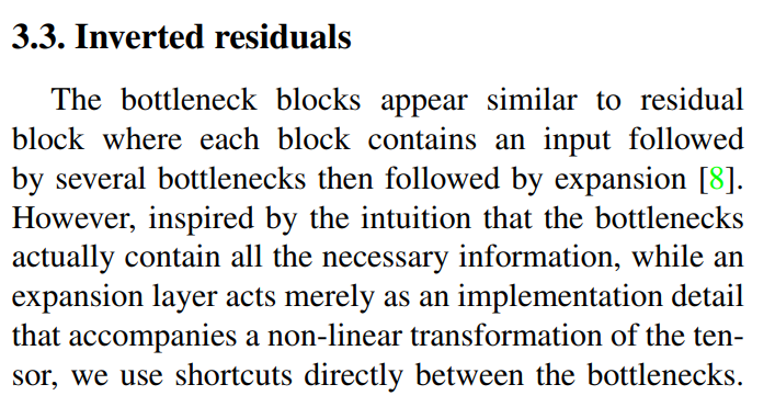
3.3. Inverted Residuals
We’ve established the two core components of the MobileNetV2 block: the narrow -> wide -> narrow structure and the linear bottleneck at the end. The final ingredient is the residual connection, also known as a “shortcut” or “skip connection,” made famous by ResNet. These connections are crucial for training very deep networks by allowing gradients to flow more easily.
The question is: where should we put the shortcut connection?
A Tale of Two Residuals
First, the authors draw a comparison to the standard residual block found in ResNet.
The bottleneck blocks appear similar to residual block where each block contains an input followed by several bottlenecks then followed by expansion [8].
A standard ResNet bottleneck block has a wide -> narrow -> wide structure. To help gradients flow, the shortcut connection skips over the narrow part and connects the two wide ends of the block. The thinking is that the wide representations contain the most information, so they should be preserved.
Inverting the Logic
MobileNetV2, however, is built on a completely different intuition.
However, inspired by the intuition that the bottlenecks actually contain all the necessary information, while an expansion layer acts merely as an implementation detail that accompanies a non-linear transformation of the tensor, we use shortcuts directly between the bottlenecks.
This is the logical conclusion of their entire theoretical argument. Let’s trace the reasoning:
- The “Manifold of Interest” is low-dimensional.
- Therefore, the narrow bottleneck layers are the most compact and complete representation of this manifold. They are the true home of the important information.
- The wide expansion layer, on the other hand, is just a temporary “safety net.” Its purpose is purely functional: to provide a high-dimensional space where
ReLUcan be applied safely. It’s an “implementation detail,” not the primary carrier of information.
Given this logic, it makes no sense to connect the wide, temporary expansion layers. It makes perfect sense to connect the narrow, information-rich bottleneck layers.
By connecting the thin input bottleneck to the thin output bottleneck, the shortcut allows the network to directly pass the core “manifold of interest” from one block to the next, while the expansion-projection part of the block learns to refine this representation.
This is why the design is called an “Inverted Residual”:
- Standard Residual (ResNet):
wide -> narrow -> widewith a shortcut between the wide layers. - Inverted Residual (MobileNetV2):
narrow -> wide -> narrowwith a shortcut between the narrow layers.
Visualizing the Inversion: Standard vs. Inverted Residuals (Figure 3)
The authors provide a clear schematic in Figure 3 to visualize the difference between the two residual block designs. Just like in Figure 2, the thickness of the blocks represents the number of channels (wide or narrow), and the hatched texture indicates a linear layer with no non-linearity.
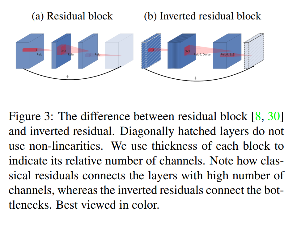
(a) The Classic Residual Block (ResNet-style)
- Structure:
wide -> narrow -> wide. - Flow: The block takes a wide input, uses a
1x1convolution to project it down to a narrow bottleneck, processes it with a3x3convolution, and then uses another1x1convolution to expand it back out to a wide representation. - Shortcut Connection: The key thing to notice is the curved arrow. The shortcut connects the two wide ends of the block. It bypasses the narrow bottleneck.
(b) The Inverted Residual Block (MobileNetV2-style)
- Structure:
narrow -> wide -> narrow. - Flow: This is the complete MobileNetV2 block. It takes a narrow input, uses a
1x1convolution to expand it to a wide intermediate representation, processes it with a3x3depthwise convolution (this is where theReLUlives), and then uses a final linear1x1convolution to project it back down to a narrow output. - Shortcut Connection: Now look at this arrow. The shortcut connects the two narrow ends of the block. It completely bypasses the wide expansion layer.
Why is the Inverted Design Better?
The authors conclude by summarizing the benefits of their new design.
The motivation for inserting shortcuts is similar to that of classical residual connections: we want to improve the ability of a gradient to propagate across multiplier layers.
First, they acknowledge that the fundamental reason for using shortcuts is the same as in ResNet: to combat the vanishing gradient problem and enable the training of much deeper networks. The shortcut provides a direct, uninterrupted path for gradients to flow backward through the network.
However, the inverted design is considerably more memory efficient (see Section 5 for details), as well as works slightly better in our experiments.
This is the punchline. The inverted design isn’t just a different way to do the same thing; it’s a better way, for two key reasons:
- Memory Efficiency: This is a huge advantage for mobile devices. Because the inputs and outputs of the block are thin, bottleneck tensors, much less memory is needed to store them for the shortcut connection. The large, intermediate tensors exist only transiently inside the block and don’t need to be kept in memory. In contrast, the classic residual block needs to keep the large, wide input tensor in memory to add it to the output later. The authors promise to elaborate on this crucial advantage in Section 5.
- Performance: The bottom line is that it simply works better. The authors state that their experiments show this inverted design leads to slightly higher accuracy than a comparable network built with standard residual blocks.
Running Time and Memory: The Payoff of the Inverted Design
We now have a complete picture of the MobileNetV2 block: an inverted residual with a linear bottleneck. But what does this mean in practice? How does it affect performance? The authors now quantify the computational cost and, more importantly, the memory efficiency of their design.
The Block Structure and Cost Formula
First, the authors formalize the structure of the block in Table 1 and provide a formula for its computational cost (measured in Multiply-Adds, or MAdds).
Table 1: The Bottleneck Residual Block
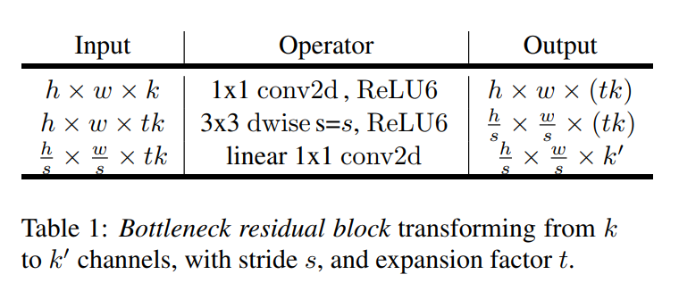
This table is a clear, step-by-step recipe for the block’s operations:
- Input: A narrow tensor with
kchannels. - Step 1 (Expansion): A
1x1convolution withReLU6expands the input totkchannels, wheretis the expansion factor. - Step 2 (Filtering): A
3x3depthwise convolution withReLU6filters this wide tensor. This is where downsampling can happen if the stridesis greater than 1. - Step 3 (Projection): A linear
1x1convolution projects the wide tensor back down to a narrow output withk'channels.
The paper then presents the formula for the total MAdds required for this block:
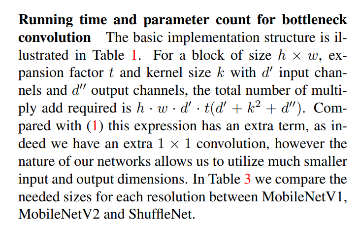
…the total number of multiply add required is h · w · d’ · t(d’ + k² + d’’).
This formula represents the sum of the costs of the three convolutions. It looks more complex than the original depthwise separable convolution formula because of the extra 1x1 expansion layer.
However, the authors make a crucial point:
…however the nature of our networks allows us to utilize much smaller input and output dimensions.
This is the key to the whole design. Even though the block has three operations instead of two, the input and output of the block (d' and d'') are the narrow bottlenecks. In contrast, the input and output of a MobileNetV1 block are the wide layers. This fundamental difference has a massive impact on memory usage, as shown in Table 3.
The Memory Efficiency Punchline (Table 3)
Table 3 is perhaps the most compelling piece of evidence for the superiority of the inverted residual design for mobile applications. It compares the maximum memory required at any point during inference for three different architectures. This “peak memory usage” is a critical bottleneck on devices with limited RAM.
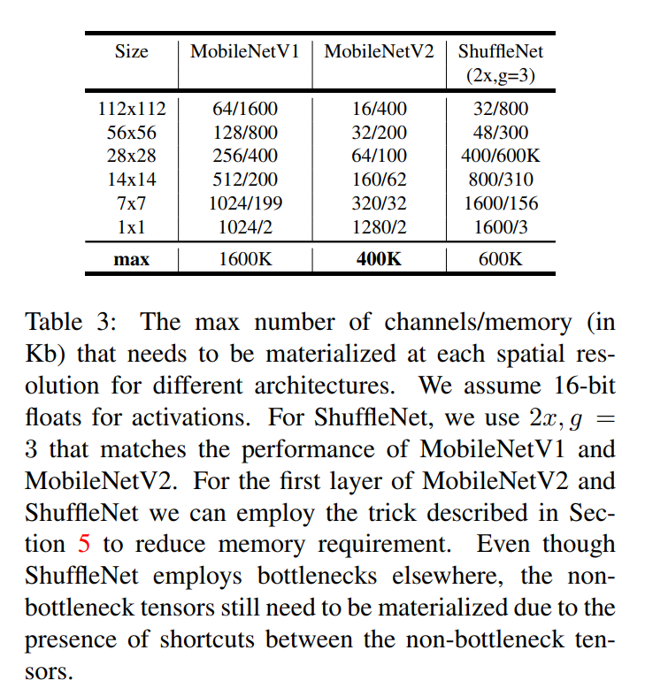
Let’s look at the results in the “max” row:
- MobileNetV1: Requires a peak of 1600 Kb of memory for activations.
- ShuffleNet (a competitor): Is much better, requiring 600 Kb.
- MobileNetV2: Requires only 400 Kb!
This is a huge win. MobileNetV2 uses 4x less peak memory than its predecessor and is 1.5x more memory-efficient than its direct competitor, ShuffleNet.
Why is it so much better? The caption of Table 3 gives us the answer, and it confirms our understanding of the residual connections: > …Even though ShuffleNet employs bottlenecks elsewhere, the non-bottleneck tensors still need to be materialized due to the presence of shortcuts between the non-bottleneck tensors.
Both MobileNetV1 and ShuffleNet use classic residual connections that link the wide layers. This means the network has to keep these large, wide activation tensors fully “materialized” (stored) in memory so it can add them back in after the block.
MobileNetV2’s inverted design, with shortcuts between the narrow bottlenecks, completely avoids this. The only tensors that need to be kept around are the small, compact bottleneck representations. The large intermediate tensor is a temporary variable that can be discarded as soon as it’s used. This is a direct and powerful consequence of the inverted residual design and a major reason for its success on mobile devices.
3.4. Information Flow Interpretation
In this final part of the theory section, the authors take a step back and offer a new perspective on their architecture. They argue that the inverted residual design has a unique and desirable property: it naturally separates the network’s capacity from its expressiveness.
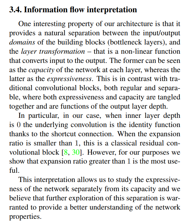
Untangling Capacity and Expressiveness
One interesting property of our architecture is that it provides a natural separation between the input/output domains of the building blocks (bottleneck layers), and the layer transformation – that is a non-linear function that converts input to the output. The former can be seen as the capacity of the network at each layer, whereas the latter as the expressiveness.
Let’s define these two key terms in the context of a MobileNetV2 block:
- Capacity: This refers to the bottleneck layers. The number of channels in these narrow input/output layers represents the total amount of information, or “capacity,” that can flow from one block to the next. It’s the information highway’s width.
- Expressiveness: This refers to the intermediate expansion layer. This is where the non-linear transformation happens. The size of this expansion (controlled by the expansion ratio
t) determines how complex and expressive the transformation can be. It’s the power of the “factory” built alongside the highway.
The authors argue that in their design, these two concepts are decoupled. You can change the expressiveness of a block (by tweaking the expansion ratio t) without changing the capacity of the information flowing between blocks.
This is in contrast with traditional convolutional blocks, both regular and separable, where both expressiveness and capacity are tangled together and are functions of the output layer depth.
In a traditional block (like in MobileNetV1 or a standard CNN), the output of the block is the result of the non-linear transformation. The number of output channels determines both the capacity (how much information is passed on) and the expressiveness (the space in which the transformation was performed). The two are fundamentally “tangled.” If you want more expressiveness, you must increase the capacity by making the output wider, which makes the whole network bigger.
The Power of Separation
This separation in MobileNetV2 provides a cleaner framework for network design and analysis.
In particular, in our case, when inner layer depth is 0 the underlying convolution is the identity function thanks to the shortcut connection. When the expansion ratio is smaller than 1, this is a classical residual convolutional block [8, 30]. However, for our purposes we show that expansion ratio greater than 1 is the most useful.
This decoupling allows for a more flexible design. The authors point out some interesting edge cases:
- If you set the expansion ratio to 0 (making the inner layer have 0 depth), the block becomes an identity function because of the residual connection. The input passes straight to the output.
- If you set the expansion ratio to a value between 0 and 1, you are effectively creating a classic ResNet-style bottleneck (
wide -> narrow -> wide). - However, the most powerful configuration, as their theory suggests, is an expansion ratio greater than 1. This is the
narrow -> wide -> narrowstructure that givesReLUthe high-dimensional safety net it needs.
This interpretation allows us to study the expressiveness of the network separately from its capacity and we believe that further exploration of this separation is warranted to provide a better understanding of the network properties.
The authors conclude by suggesting this is a promising area for future research. By cleanly separating these two fundamental properties of a network layer, their architecture might allow for a deeper and more principled understanding of how deep neural networks learn. It provides a new set of levers for researchers to pull when designing future architectures.
Why Capacity is the Narrow Bottleneck
Capacity is the maximum amount of information that is preserved and passed from one block to the next.
In MobileNetV2, the input to a block and the output from a block are the narrow bottleneck tensors. The residual connection also links these narrow tensors. Therefore, these bottlenecks act as the “information highway” of the network.
- The number of channels in the bottleneck layer is like the number of lanes on the highway.
- A bottleneck with 16 channels has a lower capacity to carry information forward than a bottleneck with 32 channels.
- The authors’ core intuition is that this highway doesn’t need to be massive, because the “manifold of interest” is low-dimensional and doesn’t take up much space. The bottleneck’s width should be just wide enough to carry this manifold.
This is the state of the network—the compressed representation of the image that is passed sequentially through the network.
Why Expressiveness is the Wider Expansion
Expressiveness (or expressive power) is the ability of a block to learn complex, non-linear functions to transform its input.
In MobileNetV2, the actual transformation happens inside the block, specifically within the wide expansion layer.
- This expansion layer is the “factory” built alongside the highway.
- The raw materials (the input bottleneck tensor) are taken off the highway and brought into this factory.
- The expansion ratio (
t) determines the size of the factory. A larger expansion ratio means a bigger factory (more channels), which provides a higher-dimensional space forReLUto perform more complex “cutting and folding” operations safely. - After the transformation, the finished goods (the output tensor) are put back onto the narrow highway (projected back down to a bottleneck) to be sent to the next block.
This is the transformation of the network—the function that modifies the state.
4. Model Architecture: Assembling the Blocks
Having established the theory and design principles behind the inverted residual and linear bottleneck, the authors now present the full, concrete architecture of MobileNetV2. This section is the recipe that puts all the pieces together.
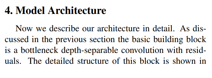
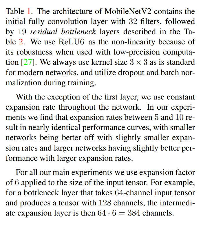
Now we describe our architecture in detail. As discussed in the previous section the basic building block is a bottleneck depth-separable convolution with residuals. The detailed structure of this block is shown in Table 1.
The overall structure is straightforward:
- A single, initial standard convolution layer.
- A main body composed of 19 inverted residual bottleneck blocks.
- A final set of layers for classification.
Let’s look at the key design choices.
Core Components and Hyperparameters
The architecture of MobileNetV2 contains the initial fully convolution layer with 32 filters, followed by 19 residual bottleneck layers described in the Table 2. We use ReLU6 as the non-linearity because of its robustness when used with low-precision computation [27]. We always use kernel size 3 × 3 as is standard for modern networks, and utilize dropout and batch normalization during training.
This paragraph outlines some standard choices:
- Non-linearity: They use
ReLU6(min(max(0, x), 6)) instead of a standardReLU. This is a practice inherited from MobileNetV1, as capping the activation value at 6 makes the model more robust when using lower-precision number formats (like 16-bit floats or 8-bit integers), which is very important for mobile inference. - Standard Practices: They use
3x3kernels for the depthwise convolutions and employ standard training techniques like dropout and batch normalization.
The All-Important Expansion Factor
Next, they discuss the key hyperparameter of their new block: the expansion factor t.
With the exception of the first layer, we use constant expansion rate throughout the network… For all our main experiments we use expansion factor of 6 applied to the size of the input tensor.
This is a crucial and simplifying design choice. Instead of tuning the expansion factor for every single layer, they found that using a constant expansion factor of t=6 works very well across the entire network.
They provide a concrete example to make this clear:
For example, for a bottleneck layer that takes 64-channel input tensor and produces a tensor with 128 channels, the intermediate expansion layer is then 64 · 6 = 384 channels.
This perfectly illustrates the narrow -> wide -> narrow flow:
- Input (Narrow): 64 channels
- Expansion (Wide):
64 * 6 = 384channels (This is where ReLU6 is applied) - Output (Narrow): 128 channels (This projection is linear)
The Blueprint: Understanding Table 2
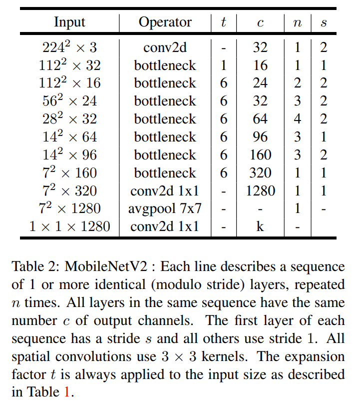
Table 2 is the definitive blueprint for the entire MobileNetV2 architecture. Each row describes a sequence of one or more identical layers. Let’s decode the columns:
t: The expansion factor for the blocks in that sequence.c: The number of output channels for the blocks. This is the “capacity” of the bottleneck.n: The number of times the block is repeated in this sequence.s: The stride. A stride of 2 (s=2) is used for downsampling, while a stride of 1 (s=1) processes features at the same resolution.
Let’s trace the information flow through the network using the table:
- Initial Layer: The network starts with a standard
conv2dwith stride 2, immediately halving the input image resolution (e.g., from 224x224 to 112x112) and creating 32 channels. - First Bottleneck: The first bottleneck block is special. It has an expansion factor of
t=1, meaning it doesn’t expand the channels at all. It simply projects the 32 input channels down to 16. - The Main Body: From here, we see a repeating pattern that is classic in CNNs:
- The network processes data at a certain resolution for
nblocks. - The first block of a new sequence (
s=2) halves the spatial resolution and increases the number of channelsc(e.g., from 56x56@24 channels to 28x28@32 channels). - The subsequent
n-1blocks (s=1) process features at this new resolution.
- The network processes data at a certain resolution for
- Final Layers: After the last bottleneck block, a
1x1convolution expands the channels to 1280. An average pooling layer then collapses the spatial dimensions to 1x1, and a final classifier layer produces the output predictions.
A Family of Models: The Trade-off Hyperparameters
One of the key strengths of the MobileNet family is that it’s not a one-size-fits-all architecture. The authors describe two simple “dials” that a developer can turn to create a wide spectrum of models, trading off accuracy for performance in a predictable way.
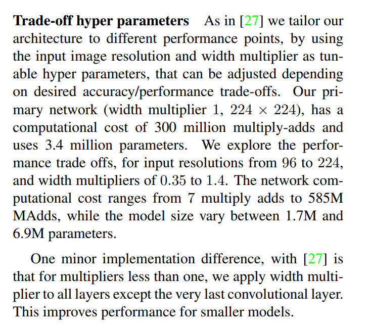
As in [27] we tailor our architecture to different performance points, by using the input image resolution and width multiplier as tunable hyper parameters, that can be adjusted depending on desired accuracy/performance trade-offs.
These are the two main levers you can pull:
- Input Image Resolution: This is straightforward. You can choose to feed the network smaller or larger images.
- Lower Resolution (e.g., 96x96): This is much faster. The network has far fewer pixels to process in the initial layers, leading to a massive reduction in computational cost. The trade-off is that the model might miss fine-grained details, leading to lower accuracy.
- Higher Resolution (e.g., 224x224): This is more computationally expensive but provides the network with more detail, which can lead to higher accuracy.
- Width Multiplier: This is a single floating-point number (e.g., 1.0, 0.75, 0.5, 1.4) that acts as a scaling factor for the number of channels (
c) in every layer of the network (as defined in Table 2).- Width Multiplier < 1.0 (e.g., 0.5): This makes the network “thinner” by halving the number of channels everywhere. This quadratically reduces the computational cost and the number of parameters, making the model much smaller and faster. The trade-off is a potential drop in accuracy, as the network has less capacity.
- Width Multiplier > 1.0 (e.g., 1.4): This makes the network “wider” by increasing the number of channels. This increases the model’s capacity and can lead to higher accuracy, at the cost of more computation and a larger model size.
A Huge Spectrum of Possibilities
By combining these two hyperparameters, you can generate a whole family of MobileNetV2 variants tailored to specific needs.
Our primary network (width multiplier 1, 224 × 224), has a computational cost of 300 million multiply-adds and uses 3.4 million parameters. We explore the performance trade offs, for input resolutions from 96 to 224, and width multipliers of 0.35 to 1.4. The network computational cost ranges from 7 multiply adds to 585M MAdds, while the model size vary between 1.7M and 6.9M parameters.
The authors provide the specs for their baseline model and then show the incredible range they can achieve:
- Baseline (1.0 width, 224x224): 300M MAdds, 3.4M parameters.
- Smallest Extreme (e.g., 0.35 width, 96x96): As low as 7M MAdds and 1.7M parameters. This is tiny and incredibly fast, suitable for the most resource-constrained environments.
- Largest Extreme (1.4 width, 224x224): Up to 585M MAdds and 6.9M parameters. This is a much more powerful model that can compete with larger architectures while still being relatively efficient.
A Minor Tweak for Smaller Models
Finally, they note one small implementation detail that improves performance for the smaller variants of the model.
One minor implementation difference, with [27] is that for multipliers less than one, we apply width multiplier to all layers except the very last convolutional layer. This improves performance for smaller models.
This is a pragmatic tweak. The final 1x1 convolution layer (the one that expands from 320 to 1280 channels in the baseline model) is responsible for creating a rich feature space for the final classifier. The authors found that for smaller models (width multiplier < 1.0), it’s beneficial to keep this final layer “wide” and not shrink it. The rich features it produces help to compensate for the reduced capacity in the rest of the network, providing a nice boost to accuracy for these smaller models.
Putting It All Together: A Visual Comparison of Architectures (Figure 4)
Figure 4 provides a concise visual summary, comparing the building blocks of four different state-of-the-art efficient architectures. This helps us appreciate the design choices made in MobileNetV2 by seeing the alternatives.
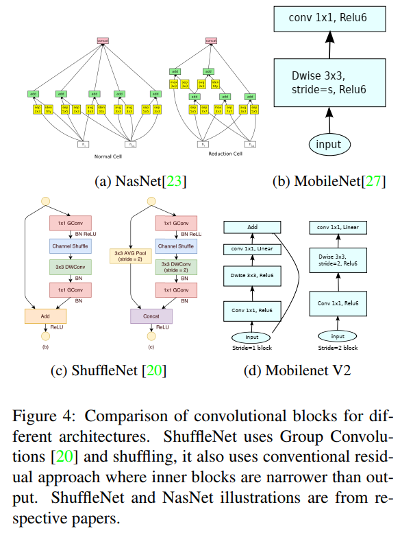
(a) NasNet: The Machine-Designed Block
- What it is: This is a block (“cell”) discovered by Neural Architecture Search (NAS). Instead of being designed by a human, it was found by an algorithm that searched through thousands of possible combinations of operations.
- Key Feature: Extreme complexity. The diagram is a complex graph of different convolutions (separable 3x3s, 5x5s) and connections.
- Design Philosophy: As we discussed in the “Related Work” section, this is the opposite of MobileNetV2’s philosophy. It prioritizes performance above all else, even if the resulting design is complex and unintuitive.
(b) MobileNetV1: The Simple Separable Block
- What it is: This is the simple, two-layer depthwise separable convolution block that started it all.
- Key Feature: Simplicity. It’s a
wide -> wideblock, consisting of a depthwise convolution followed by a pointwise convolution. - Design Philosophy: This block is all about efficiency through factorization. It’s the foundation upon which MobileNetV2 is built.
(c) ShuffleNet: The Grouped and Shuffled Block
- What it is: This is the building block of ShuffleNet, a major competitor to MobileNetV2.
- Key Feature: It uses clever operations like pointwise group convolutions (GConv) and a channel shuffle operation to create efficient, information-rich representations. It uses a standard residual connection, where the shortcut bypasses the narrow bottleneck part of the block (similar to ResNet). The block on the right also shows how it handles downsampling.
- Design Philosophy: Like MobileNetV2, this is a human-designed, intuition-driven block focused on efficiency. It just uses a different set of tricks to achieve it. The caption notes that it uses the “conventional residual approach where inner blocks are narrower than output,” highlighting its contrast with MobileNetV2’s inverted design.
(d) MobileNetV2: The Inverted Residual Block
- What it is: This is our hero block, shown in its two forms: the standard
stride=1block and the downsamplingstride=2block. - Key Features:
- Inverted Residual: The
narrow -> wide -> narrowstructure is clearly visible. - Linear Bottleneck: The final
conv 1x1, Linearlayer explicitly calls out the removal of the non-linearity. - Shortcut Connection: The
Addoperation connects the narrow input to the narrow output, bypassing the wide expansion.
- Inverted Residual: The
- Design Philosophy: This block embodies all the principles we’ve discussed: efficiency from depthwise separation, information preservation via linear bottlenecks, safe non-linearity via high-dimensional expansion, and memory efficiency via inverted residuals.
5. Implementation Notes: A Memory Efficiency Masterclass
The authors have already shown that their inverted residual design leads to lower peak memory usage because the shortcuts connect the narrow bottlenecks (as seen in Table 3). In this section, they reveal an additional, powerful implementation trick that the block’s unique structure enables, further slashing memory consumption during inference.
This is a bit technical, but it’s a beautiful example of how thoughtful architectural design can unlock significant performance gains in practice.
5.1. Memory Efficient Inference
The General Problem: Minimizing Peak Memory
First, the authors set the stage by describing how deep learning frameworks generally handle memory.
A standard efficient implementation of inference… builds a directed acyclic compute hypergraph G, consisting of edges representing the operations and nodes representing tensors… The computation is scheduled in order to minimize the total number of tensors that needs to be stored in memory.
Think of a neural network as a recipe. The “nodes” are the ingredients (the tensors/feature maps), and the “edges” are the steps (the convolutions, additions, etc.). A framework like TensorFlow or PyTorch acts as the chef. The chef’s job is to follow the recipe in an order that minimizes the amount of counter space (RAM) needed at any single moment. This maximum counter space required is the peak memory usage. For a mobile phone with limited RAM, keeping this peak low is critical.
The MobileNetV2 Solution: Compute-in-Parts
The MobileNetV2 block’s structure allows for a particularly clever scheduling trick. The authors first represent their block as a composition of three operators: F(x) = [A ◦ N ◦ B]x.
Bis the initial linear1x1expansion convolution.Nis the non-linear, per-channel transformation (the3x3depthwise convolution +ReLU6).Ais the final linear1x1projection convolution.
The key to the entire trick lies in the properties of the middle operator, N. Because it is per-channel, it can be broken up into smaller pieces. This allows the entire block function F(x) to be represented as a sum:
F(x) = Σ (A_i ◦ N ◦ B_i)(x)
What does this mean in practice?
Instead of calculating the entire massive intermediate tensor from the expansion layer all at once, you can compute it in smaller chunks and accumulate the result.
Let’s use an analogy:
- Standard Method: To calculate
100 * 50, you first compute the intermediate result5000(materializing the large tensor), and then you use that5000in the next step. You need enough space to hold the number5000. - MobileNetV2’s “t-way split” Method: You can instead compute this as
(10 * 50) + (10 * 50) + ...(10 times). You only need enough memory to hold the intermediate result500and a running total. You compute500, add it to the total, and then discard it to compute the next500. The peak memory required is much smaller.
This is exactly what the authors propose. By splitting the computation into t parts (where t is a small number like 4), they only need to keep 1/t of the large intermediate tensor in memory at any given time.
The algorithm is based on the fact that the inner tensor I can be represented as concatenation of t tensors… by accumulating the sum, we only require one intermediate block… to be kept in memory at all times.
The Practical Trade-Off
This memory-saving trick doesn’t come for free. There is a trade-off with runtime speed.
…in existing implementations we find that replacing one matrix multiplication with several smaller ones hurts runtime performance due to increased cache misses.
Modern CPUs and GPUs are highly optimized for performing single, large matrix multiplications. Breaking one big operation into many smaller ones can be less efficient because the hardware has to constantly fetch new, small chunks of data from memory, leading to “cache misses” which slow down the computation.
Therefore, the authors suggest a pragmatic compromise:
We find that this approach is the most helpful to be used with t being a small constant between 2 and 5.
By using a small split factor, you can get a significant reduction in memory usage while only taking a minor hit on runtime performance. This provides a great balance for on-device applications, where both memory and latency are critical.
This entire section demonstrates that the benefits of the inverted residual structure go beyond theory; its specific design directly enables powerful, practical optimizations that are a huge win for mobile deep learning.
6. Experiments: Putting Theory to the Test
After laying out a compelling theoretical argument and a novel architecture, the authors now present the empirical evidence to back up their claims. They evaluate MobileNetV2 across a wide range of tasks and directly test their core hypotheses through ablation studies.
6.1. ImageNet Classification: The Main Event
The standard benchmark for any new vision architecture is its performance on the massive ImageNet dataset.
Training Setup: The authors use a standard training regimen with TensorFlow, the RMSProp optimizer, and a typical learning rate schedule. This ensures their results are comparable to other papers and not the result of some exotic training trick.
Results (Figure 5 and Table 4): The results are shown in a performance curve (Figure 5) that plots accuracy against computational cost (MAdds). This is the best way to evaluate an efficient network.
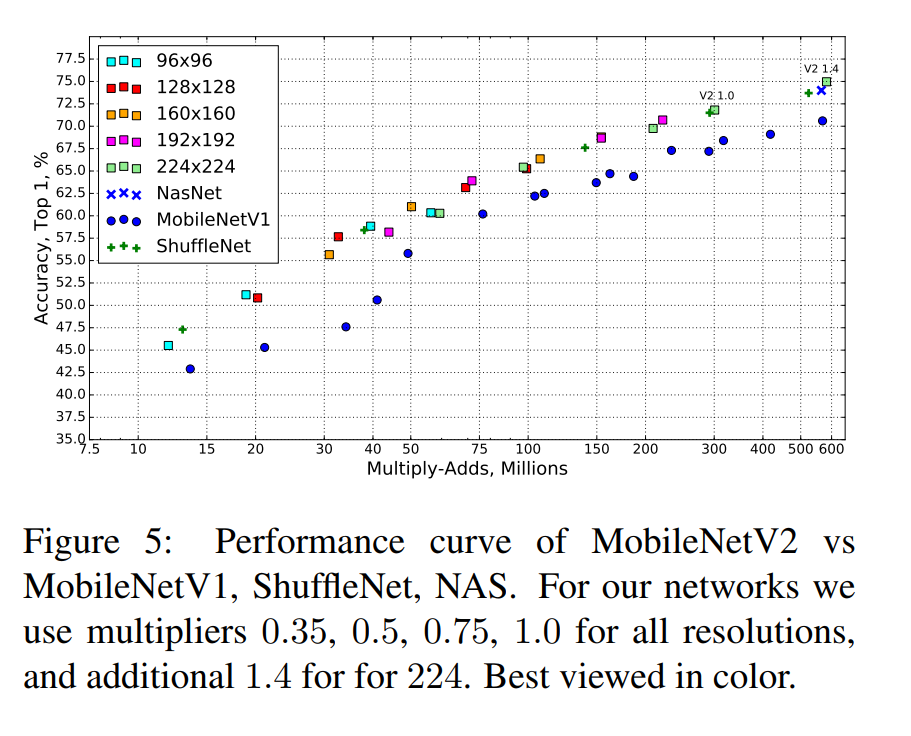
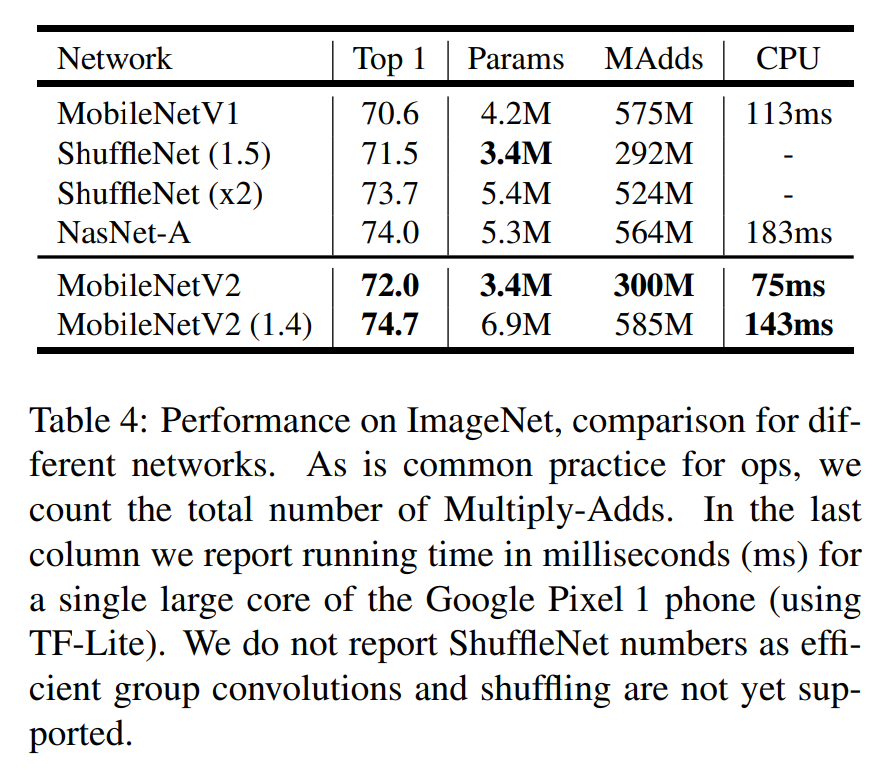
- The Punchline: The MobileNetV2 curve is consistently higher and to the left of the curves for MobileNetV1 and ShuffleNet. This is a decisive win. It means that:
- For any given computational budget (a vertical line on the graph), MobileNetV2 achieves higher accuracy.
- To achieve a target accuracy level (a horizontal line), MobileNetV2 requires significantly less computation.
- Concrete Numbers (Table 4): Let’s compare the baseline 1.0 models:
- MobileNetV1: 70.6% accuracy @ 575M MAdds
- MobileNetV2: 72.0% accuracy @ 300M MAdds
This is an incredible result. MobileNetV2 is 1.4% more accurate while using almost half the computation. It also achieves this with fewer parameters (3.4M vs 4.2M) and is significantly faster on a real Google Pixel 1 phone (75ms vs 113ms).
6.2. Object Detection: Beyond Classification with SSDLite
Next, the authors test MobileNetV2 as a “backbone” feature extractor for the task of object detection on the COCO dataset.
The SSDLite Innovation: A key contribution here is a new mobile-friendly detector they call SSDLite. They took the popular Single Shot Detector (SSD) and replaced all the standard convolutions in its prediction layers with depthwise separable convolutions. As shown in Table 5, this simple change dramatically reduces the parameter count and computational cost of the detector head itself.
Results (Table 6): The results are a massive success for the combination of MobileNetV2 and SSDLite.
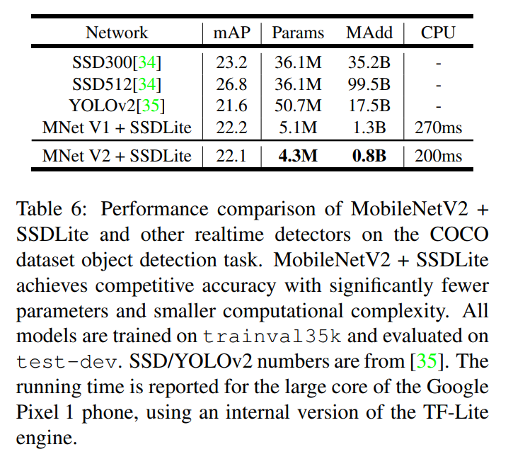
Comparison to YOLOv2: This is the most stunning comparison. YOLOv2 was a very popular real-time detector.
- Accuracy: MobileNetV2+SSDLite is slightly more accurate (22.1 vs 21.6 mAP).
- Efficiency: It is ~20x more computationally efficient (0.8B vs 17.5B MAdds).
- Size: It is ~10x smaller (4.3M vs 50.7M parameters).
6.3. Semantic Segmentation: Painting a Picture
The third test is on semantic segmentation using the powerful DeepLabv3 framework on the PASCAL VOC dataset.
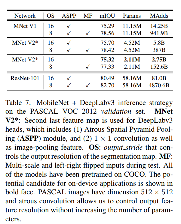
Results (Table 7): The story is consistent. MobileNetV2 proves to be a much more efficient feature extractor than both MobileNetV1 and the much larger ResNet-101, without a major sacrifice in accuracy (mIOU). The authors identify a specific configuration (highlighted in bold in the table) that achieves a very strong 75.32% mIOU with only 2.75B MAdds, making it a prime candidate for on-device segmentation tasks.
6.4. Ablation Studies: Proving the “Why”
This is arguably the most important part of the experiments section. Here, the authors systematically test their core architectural innovations to prove that their design choices were indeed the right ones.
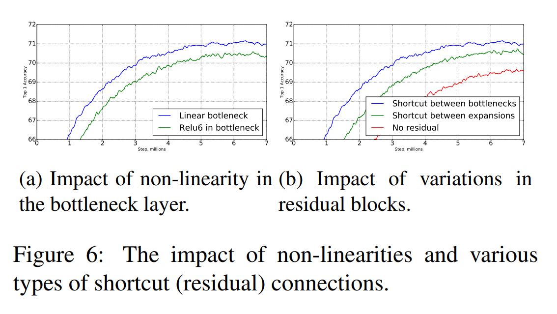
Experiment 1: The Importance of Linear Bottlenecks (Figure 6a)
- Question: Is it really necessary to remove the
ReLUfrom the bottleneck layers? - Test: They trained two models: the standard MobileNetV2 with linear bottlenecks, and a version where a
ReLU6was added back into the bottlenecks. - Result: The model with non-linear bottlenecks (
ReLU6 in bottleneck) performed significantly worse, dropping by about 1% in accuracy. - Conclusion: This is powerful empirical evidence for their main theoretical claim. Adding a non-linearity to a low-dimensional space destroys information and hurts performance.
Experiment 2: The Importance of Inverted Residuals (Figure 6b)
- Question: Is the
narrow -> wide -> narrowstructure with shortcuts between the narrow layers actually better? - Test: They compared their standard design (“Shortcut between bottlenecks”) to a more traditional design with shortcuts connecting the wide expansion layers (“Shortcut between expansions”).
- Result: The inverted residual structure performed better.
- Conclusion: This validates their intuition. Connecting the information-rich bottlenecks is not only more memory-efficient but also leads to higher accuracy.
7. Conclusions and Future Work
The final section of the paper brings everything together, summarizing the key contributions and pointing towards interesting directions for future research.
A Simple, Powerful, and Efficient Building Block
We described a very simple network architecture that allowed us to build a family of highly efficient mobile models. Our basic building unit, has several properties that make it particularly suitable for mobile applications. It allows very memory-efficient inference and relies utilize standard operations present in all neural frameworks.
The authors restate the core of their contribution: a new architectural building block—the inverted residual with a linear bottleneck—that is simple yet powerful. They re-emphasize the key practical advantages that make it so well-suited for on-device applications:
- Memory Efficiency: The inverted residual structure, with shortcuts between narrow bottlenecks, dramatically reduces the peak memory required during inference.
- Simplicity: The block is built entirely from standard, highly-optimized operations, meaning it can be deployed easily in any modern deep learning framework without needing custom code.
State-of-the-Art Performance Across the Board
The conclusion then summarizes the impressive empirical results:
For the ImageNet dataset, our architecture improves the state of the art for wide range of performance points.
For object detection task, our network outperforms state-of-art realtime detectors on COCO dataset both in terms of accuracy and model complexity. Notably, our architecture combined with the SSDLite detection module is 20× less computation and 10× less parameters than YOLOv2.
This is a concise but powerful summary of their success. MobileNetV2 isn’t just a theoretical curiosity; it delivered state-of-the-art results on multiple, challenging, large-scale benchmarks. The 20x efficiency gain over YOLOv2 is a particularly stunning achievement that had a major impact on the field of real-time object detection.
A New Direction for Research: Decoupling Capacity and Expressiveness
Finally, the authors look to the future, highlighting what they believe is the most interesting theoretical contribution of their work.
On the theoretical side: the proposed convolutional block has a unique property that allows to separate the network expressiveness (encoded by expansion layers) from its capacity (encoded by bottleneck inputs). Exploring this is an important direction for future research.
This is the “Information Flow Interpretation” from Section 3.4. The authors believe that their design, which cleanly separates the volume of information flowing through the network (capacity) from the complexity of the transformations applied to it (expressiveness), is a valuable new paradigm. It provides a cleaner framework for analyzing and designing neural networks, and they encourage the research community to explore this idea further.