A Deep Dive into Fully Convolutional Networks for Semantic Segmentation

A detailed, page-by-page breakdown of the Fully Convolutional Networks paper, explaining how to build efficient neural networks for semantic segmentation.

The paper on our reading list is foundational paper in modern computer vision: “Fully Convolutional Networks for Semantic Segmentation” by Long, Shelhamer, and Darrell from UC Berkeley. This 2015 paper was a game-changer, fundamentally shifting how deep learning models handle tasks that require pixel-level understanding.e

Diving into the Abstract (Section: Abstract)

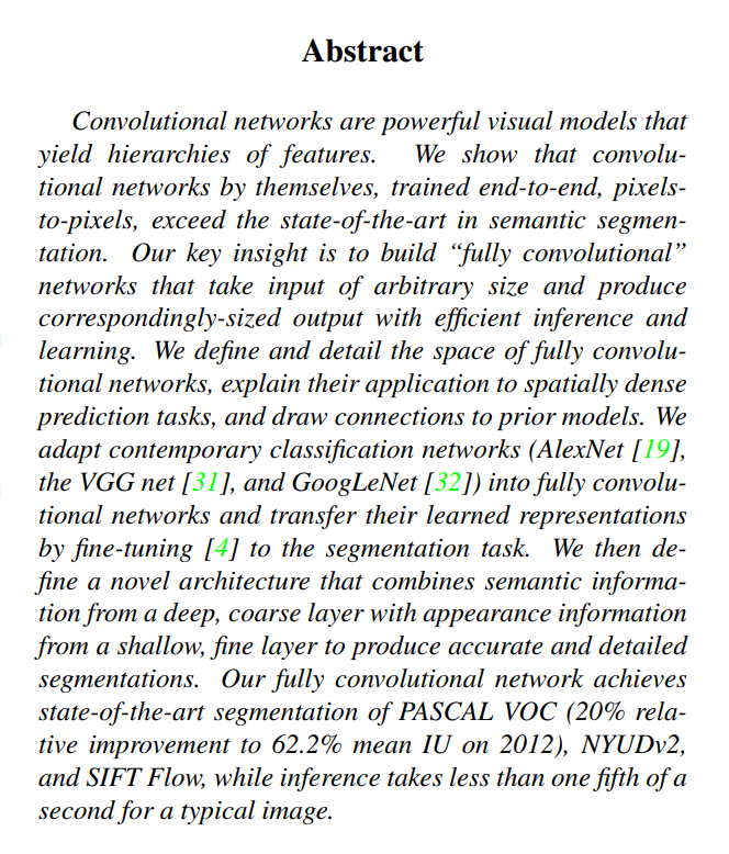
What’s the Problem? Semantic Segmentation.

First, the authors state their goal is to tackle semantic segmentation. What is that?

Imagine you show a computer a photo of a cat sitting on grass.

• Image Classification would say: “This is an image of a cat.”
• Object Detection would say: “There is a cat inside this bounding box.”
• Semantic Segmentation goes a step further. It says: “These exact pixels belong to a cat, and these other pixels belong to grass.”

It’s about understanding an image at the most granular level, classifying every single pixel. This is what the paper calls a “spatially dense prediction task.”

The “Key Insight”: Going Fully Convolutional

Before this paper, top-performing neural networks for vision tasks, like AlexNet or VGG, were primarily classifiers. They would take an image (usually of a fixed size, like 224x224 pixels) and shrink it down through a series of convolutional and pooling layers until it was small enough to be fed into a few final “fully connected” layers, which would then output a single classification (e.g., “cat,” “dog,” “car”).

The problem is that those final fully connected layers discard all spatial information. They know what is in the image, but they’ve lost track of where it is.

The authors’ “key insight” is to get rid of these fully connected layers and replace them with convolutional layers. A network composed entirely of convolutional-style layers is what they call a “fully convolutional” network (FCN). This simple but profound change has two immediate benefits mentioned in the abstract:

1. It can process images of any size. Since a convolution is just a filter that slides over the input, it doesn’t care if the image is 200x200 or 1000x800.
2. It produces an output map, not just a single number. The output is a “correspondingly-sized” heatmap that preserves spatial dimensions, which is exactly what we need for segmentation.

Building on the Shoulders of Giants: Transfer Learning

The authors didn’t start from scratch. They took the powerful, pre-trained classification networks of the day (AlexNet, VGGNet, GoogLeNet) and “adapted” them. These networks had already learned a rich “hierarchy of features” from being trained on the massive ImageNet dataset. They knew how to recognize edges, textures, shapes, and object parts.

The authors cleverly repurposed this knowledge. They performed a kind of “network surgery”: they chopped off the final classification layers and converted the remaining ones into an FCN. They then “fine-tuned” this modified network on the segmentation task. This is a classic example of transfer learning, and it’s far more effective than trying to train a deep network from zero.

The Second Big Idea: Combining “What” with “Where”

The abstract hints at another crucial contribution: a “novel architecture.” Deep in a neural network, the features are highly semantic but spatially coarse.

The network might know there’s a face in the image, but the feature map is so small that it can’t pinpoint the exact location of the nose. Conversely, the early layers of the network have very precise spatial information (fine details, sharp edges) but don’t know what they’re looking at.

Tip

As we go deeper into the network, our understanding of WHAT is in the image gets better (e.g., “I’m confident this is a cat face”), but our knowledge of WHERE it is located gets worse (e.g., “It’s somewhere in this big block of pixels”).

The authors’ new architecture combines this “semantic information from a deep, coarse layer with appearance information from a shallow, fine layer.” This allows the network to make predictions that are both semantically meaningful (it knows this is a car) and spatially precise (it knows exactly where the car’s boundary is). We’ll see later in the paper that they accomplish this with an elegant mechanism called “skip connections.”

The Results: State-of-the-Art and Fast

Finally, the abstract delivers the punchline. Their method works, and it works extremely well.

• It achieved state-of-the-art results on standard benchmark datasets (PASCAL VOC, NYUDv2, SIFT Flow).
• The improvement was significant: a 20% relative jump on the important PASCAL VOC 2012 benchmark. In deep learning research, that’s a massive leap, not an incremental improvement.
• It was also fast. At less than a fifth of a second per image, it was practical for real-world use.

1: Introduction

Now that we have the big picture from the Abstract, the Introduction begins to fill in the details. The authors start by framing their work as a natural next step in the evolution of deep learning, moving from coarse, image-level tasks to fine, pixel-level ones.

Let’s look at the first two paragraphs of the introduction. The first is a general statement, and the second (the one you’ve highlighted) is the core thesis.

Convolutional networks are driving advances in recognition. Convnets are not only improving for whole-image classification [19, 31, 32], but also making progress on local tasks with structured output. These include advances in bounding box object detection [29, 12, 17], part and keypoint prediction [39, 24], and local correspondence [24, 9].

The natural next step in the progression from coarse to fine inference is to make a prediction at every pixel…

This sets up their key contribution, which they detail in the next paragraph:

This paragraph is packed with crucial concepts. Let’s break it down sentence by sentence.

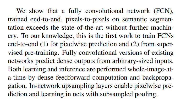
1. The Main Claim: Simple and State-of-the-Art

“We show that a fully convolutional network (FCN), trained end-to-end, pixels-to-pixels on semantic segmentation exceeds the state-of-the-art without further machinery.”

Let’s define these terms:

• End-to-end: This means the model is a single, unified system. You feed it raw pixels, and it directly outputs the final segmentation map. The entire network, from the first layer to the last, is trained together with a single learning objective. This is in stark contrast to previous methods that were often complex, multi-stage pipelines.
• Pixels-to-pixels: This is a more specific way of saying “end-to-end” for this task. The input is a grid of pixels, and the output is a corresponding grid of pixel-class labels.
• Without further machinery: This is a key point. Before FCN, state-of-the-art systems were often Frankenstein’s monsters. They would use a CNN as a feature extractor, then bolt on other complex components (“machinery”) like superpixel generation, region proposal methods, or post-processing with Conditional Random Fields (CRFs) to clean up the final output. The authors are claiming their single, elegant FCN can beat these complicated systems on its own.

2. The Novelty: What Makes This “First”?

“To our knowledge, this is the first work to train FCNs end-to-end (1) for pixelwise prediction and (2) from supervised pre-training.”

They are claiming two key “firsts”:

1. First to train an FCN end-to-end for this task: While people had used convolutional networks to produce heatmaps before (e.g., for sliding-window detection), the authors argue they are the first to set up a training procedure that learns to produce dense, pixel-level predictions directly. The learning process itself is novel.
2. First to do it from supervised pre-training: This is the transfer learning magic we discussed earlier. Previous attempts at segmentation with CNNs often used small networks trained from scratch. The authors were the first to successfully adapt the giant, powerful networks pre-trained on ImageNet for classification and fine-tune them for the segmentation task. This gave them a massive head start in feature representation.

3. The “How-To”: The Mechanics of FCNs

“Fully convolutional versions of existing networks predict dense outputs from arbitrary-sized inputs. Both learning and inference are performed whole-image-at-a-time… In-network upsampling layers enable pixelwise prediction and learning in nets with subsampled pooling.”

This part explains how it all works.

• Dense outputs from arbitrary-sized inputs: This is the direct result of replacing fully connected layers with convolutions. The network is no longer constrained to a fixed input size and naturally produces a spatial output map (a “dense output”).
• Whole-image-at-a-time: This is a major efficiency win. The common alternative was patchwise training, where you’d cut the big input image into thousands of small patches, feed each patch through the network individually to classify its center pixel, and then stitch the results together. This is incredibly slow and redundant because the network re-computes features for overlapping regions again and again. FCNs process the entire image in one go, sharing computation across all “patches” implicitly. This is what they mean by “dense feedforward computation and backpropagation.”
• In-network upsampling layers: Here they hint at the solution to the “What vs. Where” problem. As we discussed, pooling layers (“subsampled pooling”) shrink the feature maps, making them spatially coarse. To get back to the original image resolution for a final pixel-wise prediction, they need to upsample. Instead of using a simple, fixed method after the network, they build learnable upsampling layers inside the network. This allows the FCN to learn how to best create a fine-grained prediction from coarse features, all within that end-to-end training framework.

A Departure from Complexity

Having laid out their core idea, the authors now draw a sharp contrast between their elegant, unified approach and the complex, multi-stage pipelines that were common at the time.

This method is efficient, both asymptotically and absolutely, and precludes the need for the complications in other works. Patchwise training is common [27, 2, 8, 28, 11], but lacks the efficiency of fully convolutional training. Our approach does not make use of pre- and post-processing complications, including superpixels [8, 16], proposals [16, 14], or post-hoc refinement by random fields or local classifiers [8, 16]. Our model transfers recent success in classification [19, 31, 32] to dense prediction by reinterpreting classification nets as fully convolutional and fine-tuning from their learned representations. In contrast, previous works have applied small convnets without supervised pre-training [8, 28, 27].

This paragraph is a list of techniques that FCN makes obsolete. Let’s quickly define these “complications”:

• Patchwise training: We’ve already discussed this. Instead of processing a whole image at once, these methods would classify one small image patch at a time. The authors correctly point out this is highly inefficient.
• Pre- and post-processing: This refers to steps taken before the network sees the data or after it makes a prediction. The authors’ method is “end-to-end,” meaning no extra steps are needed.
• Superpixels: A pre-processing step where you group pixels into small, perceptually meaningful regions (superpixels). The network would then classify these superpixels instead of individual pixels. This adds complexity and can introduce errors if the initial grouping is bad.
• Proposals (or Region Proposals): These are “guesses” for where objects might be in an image, often generated by a separate algorithm. This was a core component of famous models like R-CNN. The network’s job was to classify these proposed regions, not the whole image.
• Post-hoc refinement by random fields: “Post-hoc” means “after the fact.” After the network made a raw, often noisy prediction, a separate model like a Conditional Random Field (CRF) would be used to clean it up, making sure neighboring pixels have similar labels. While effective, this is a separate optimization step, breaking the “end-to-end” learning principle.

The final two sentences of the paragraph reiterate their key advantages: they use transfer learning from large, pre-trained classification networks, whereas previous approaches often used smaller, custom networks trained from scratch, which were far less powerful.

Solving the “What vs. Where” Dilemma

Now we get to the heart of the architectural challenge. The authors formally state the core tension we discussed earlier and introduce their solution.

Semantic segmentation faces an inherent tension between semantics and location: global information resolves what while local information resolves where. Deep feature hierarchies jointly encode location and semantics in a local-to-global pyramid. We define a novel “skip” architecture to combine deep, coarse, semantic information and shallow, fine, appearance information in Section 4.2 (see Figure 3).

This is the most critical paragraph in the introduction.

• “The tension between semantics and location”: This is the “What vs. Where” problem.
  • Global information resolves what: To know that you’re looking at a “bicycle,” you need to see the whole object—the wheels, handlebars, and frame together. This holistic, big-picture view comes from the deep layers of the network, which have a large “receptive field.”
  • Local information resolves where: To know the precise boundary between the bicycle’s tire and the road, you need to look at a very small, high-resolution patch of pixels. This fine-grained detail is only available in the shallow, early layers of the network.
• The Solution: A “skip” architecture: How do you get the best of both worlds? The authors propose a “skip” architecture. The name is descriptive: they create connections that skip over intermediate layers of the network. These skip connections pipe the fine-grained spatial information from the early layers directly to the deep layers. The deep layers can then use this detailed map to refine their coarse semantic predictions, resulting in a final segmentation that is both accurate (knows it’s a bicycle) and precise (knows exactly where the edges are).

The Road Ahead

The introduction concludes with a standard roadmap, outlining the structure of the rest of the paper.

In the next section, we review related work on deep classification nets, FCNs, and recent approaches to semantic segmentation using convnets. The following sections explain FCN design and dense prediction tradeoffs, introduce our architecture with in-network upsampling and multilayer combinations, and describe our experimental framework. Finally, we demonstrate state-of-the-art results on PASCAL VOC 2011-2, NYUDv2, and SIFT Flow.

This tells us what’s coming: a review of prior work, a technical deep-dive into FCNs and their architecture, experimental details, and finally, the impressive results.

With the introduction complete, we now have a solid foundation for understanding the rest of this landmark paper. Next, we’ll dive into the Related Work section.

2. Related Work

In this section, the authors map out the landscape of ideas that FCN is built on and competes with. They organize the discussion into a few key areas.

The Foundations: Classification and Transfer Learning

Our approach draws on recent successes of deep nets for image classification [19, 31, 32] and transfer learning [4, 38]. Transfer was first demonstrated on various visual recognition tasks [4, 38], then on detection, and on both instance and semantic segmentation in hybrid proposal-classifier models [12, 16, 14]. We now re-architect and fine-tune classification nets to direct, dense prediction of semantic segmentation…

This first paragraph acknowledges the two giant pillars their work rests on:

1. Powerful Classification Networks: The success of AlexNet, VGGNet, and GoogLeNet on the ImageNet classification challenge provided a set of incredibly powerful, pre-trained feature extractors.
2. Transfer Learning: The idea of taking a network trained for one task (like classification) and fine-tuning it for another (like detection or segmentation) was already established.

Their key contribution, they restate, is to re-architect these nets to perform segmentation directly, rather than using them as a component in a more complex “hybrid” system.

The History of “Fully Convolutional Networks”

Here, the authors show that the idea of a network made purely of convolutional layers isn’t entirely new, but its application and training for dense prediction is.

To our knowledge, the idea of extending a convnet to arbitrary-sized inputs first appeared in Matan et al. [25], which extended the classic LeNet [21] to recognize strings of digits… Wolf and Platt [37] expand convnet outputs to 2-dimensional maps of detection scores…

They give credit to very early work from the 90s that used the fully convolutional property for simple tasks like reading multiple digits in a row.

Fully convolutional computation has also been exploited in the present era… by Sermanet et al. [29], Pinheiro and Collobert [28], and Eigen et al. [5]… Fully convolutional training is rare, but used effectively by Tompson et al. [35] to learn an end-to-end part detector…

They acknowledge that more recent works also used fully convolutional inference (the forward pass), most famously OverFeat by Sermanet et al. for sliding-window detection. However, they point out that fully convolutional training (learning the weights this way) is rare. They cite one example in pose estimation but note the authors didn’t analyze or generalize the method.

Alternatively, He et al. [17] discard the non-convolutional portion of classification nets to make a feature extractor. They combine proposals and spatial pyramid pooling… this hybrid model cannot be learned end-to-end.

This is an important contrast. Another very popular paper at the time, SPP-Net (He et al.), also solved the fixed-input-size problem of classifiers, but in a different way. The authors draw a clear line: SPP-Net is a “hybrid model” that still relies on other components (like proposals) and cannot be learned end-to-end. This highlights the elegance and unity of their own FCN approach.

The Contemporaries: “Dense Prediction with Convnets”

This is where they size up their direct competition in the segmentation space. They list several techniques that were common in other contemporary methods and implicitly state that their method doesn’t need them.

Several recent works have applied convnets to dense prediction problems… Common elements of these approaches include

• small models restricting capacity and receptive fields;
• patchwise training…
• post-processing by superpixel projection, random field regularization…
• input shifting and output interlacing for dense output… (shift-and-stitch)
• multi-scale pyramid processing…
• saturating tanh nonlinearities…
• ensembles…

…whereas our method does without this machinery.

They are essentially summarizing the entire field’s bag of tricks and then stating, “We don’t need any of that.” They do, however, note that they will analyze some of these ideas, like patchwise training and “shift-and-stitch” (a clever trick for getting higher-resolution output by running the model on slightly shifted inputs), from the perspective of their FCN framework.

The Final Showdown: The State-of-the-Art

Finally, they name their two main rivals for the state-of-the-art crown on the PASCAL VOC dataset.

Hariharan et al. [16] and Gupta et al. [14] likewise adapt deep classification nets to semantic segmentation, but do so in hybrid proposal-classifier models. These approaches fine-tune an R-CNN system… Neither method is learned end-to-end.

They achieve state-of-the-art results on PASCAL VOC segmentation… so we directly compare our standalone, end-to-end FCN to their semantic segmentation results in Section 5.

This paragraph sets up the final benchmark comparison. The reigning champions, SDS (Hariharan et al.), use a complex, multi-stage R-CNN-based pipeline. It’s powerful, but it’s slow and definitely not “end-to-end.”

3. Fully Convolutional Networks

Section 3 is the technical heart of the paper, where the authors formally define what a Fully Convolutional Network is and how it works. They start by reviewing the fundamental building blocks.

This first paragraph is a concise review of the core data structure inside a CNN. Let’s break it down.

The Data as a 3D Volume

The authors’ first point is that data inside a CNN is not a flat list of numbers; it’s a 3D block, or a “volume,” with dimensions of height (h), width (w), and depth (d).

• h & w (Spatial Dimensions): This is straightforward. It’s the “grid” of the image or feature map.
• d (Feature/Channel Dimension): This is the most interesting part.
  • For the very first layer (the input image), d is the number of color channels. For a standard color photo, d=3 (Red, Green, Blue).
  • For deeper layers, d represents the number of features or filters that the layer has learned. For example, a layer might have d=256, meaning it has learned 256 different feature detectors. One feature detector might look for vertical edges, another might look for a specific texture, and a third might look for a reddish-blue color combination.

So, a CNN takes a 3D volume (the input image) and transforms it into a series of other 3D volumes (the feature maps).

What is a Receptive Field?

This is arguably the most important concept in this paragraph.

“Locations in higher layers correspond to the locations in the image they are path-connected to, which are called their receptive fields.”

A single “pixel” or neuron in a deep feature map doesn’t just see one pixel from the original input. It sees a whole region. The receptive field is the specific patch of the original input image that influences the value of that single neuron.

Think of it like this:

• A neuron in the first convolutional layer might look at a tiny 3x3 patch of pixels from the input image. Its receptive field is 3x3.
• A neuron in the second layer looks at a 3x3 patch of neurons from the first layer. But since each of those neurons saw a 3x3 patch of the input, this second-layer neuron is actually seeing a larger 5x5 region of the original input. Its receptive field is 5x5.

As you go deeper, the receptive field size grows. A neuron deep in the network might have a receptive field of 200x200 pixels. This is how CNNs build up a hierarchical understanding:

• Shallow layers have small receptive fields. They focus on local details like edges and corners (high-precision “where” information).
• Deep layers have large receptive fields. They can see enough of the image to recognize complex objects like faces or cars (high-level “what” information).

Receptive Field in the Convolutional Networks

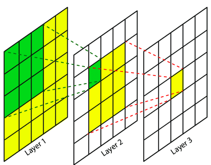
Image Source: Receptive Field in the Convolutional Networks

After establishing the basic data structure (the 3D volume), the authors now get into the mathematical properties of the layers themselves. This part is a little dense, but it’s the foundation for everything that follows.

Let’s unpack this step-by-step.

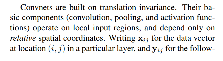
1. The Core Principle: Translation Invariance

The most important sentence is the first one: “Convnets are built on translation invariance.” (Technically, it’s equivariance, but the general idea is the same).

• Translation means moving something without rotating or resizing it.
• Invariance means that something doesn’t change.

So, “translation invariance” means that if you take an object (like a cat) in an image and move it to a different location, the network should still recognize it as a cat. The network’s “cat detector” works everywhere in the image.

How does it achieve this? The next line explains: the operations depend only on relative spatial coordinates. A filter doesn’t know if it’s at position (x=10, y=20) or (x=300, y=400). It only knows the pattern of values in its immediate neighborhood—the pixels to its “top-left,” “bottom-right,” etc. The same filter weights are applied at every single location, which is what gives it this powerful property.

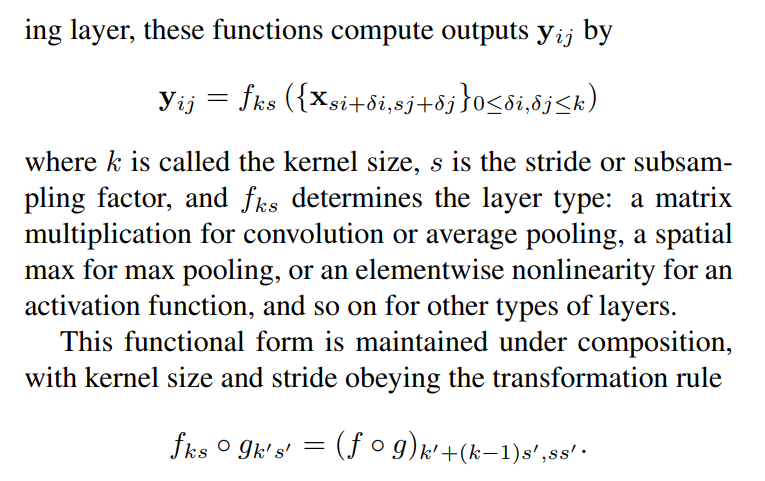
2. The General Equation for a CNN Layer

The equation y_ij = f_ks(...) looks intimidating, but it’s just a general way to write down what any CNN layer does. Let’s translate it into English:

“The output value at a single location y_ij in this layer is calculated by a function f, which takes in a small patch of input values from the previous layer x.”

Let’s look at the pieces:

• y_ij: A single output value (or vector of features) at coordinate (i, j).
• x: The input from the previous layer.
• f_ks: The function the layer performs.
  • It could be max pooling (find the maximum value in the input patch).
  • It could be convolution (perform a weighted sum of the input patch).
  • It could be ReLU (an activation function applied to each element).
• k (kernel size): How big is the input patch we’re looking at? A k=3 means we’re looking at a 3x3 neighborhood.
• s (stride): How far do we jump in the input to calculate the next output? A s=1 means we slide the window one pixel at a time. A s=2 means we jump two pixels, effectively downsampling the output.
• The complicated-looking x_si+δi, sj+δj is just the math for “grab the input patch of size k centered around the location (si, sj).”

3. The Power of Composition

The paragraph concludes with another important mathematical property.

This functional form is maintained under composition, with kernel size and stride obeying the transformation rule

f_ks ◦ g_k’s’ = (f ◦ g)_{k’+(k-1)s’, ss’}

This is a fancy way of saying: “When you stack these layers, they compose in a predictable way.”

If you have one layer g followed by another layer f, the combination of the two (f ◦ g) acts like a single, larger layer of the same type. This new super-layer has a new, larger effective kernel size and a new, larger effective stride.

• New stride (ss'): This is simple. If you have a layer with stride 2, and you stack another layer with stride 2 on top, the total stride from the input of the first layer to the output of the second is 2 * 2 = 4. The strides multiply.
• New kernel size (k' + (k-1)s'): This is the formula for calculating the growth of the receptive field! It tells you exactly how big a patch of the original input a neuron sees after two layers.

The key takeaway is that the fundamental nature of the computation doesn’t change as you go deeper. You are just creating a filter with a larger and larger receptive field. This mathematical elegance is what makes deep CNNs so powerful and analyzable.

The Efficiency of Whole-Image Training

After defining the mathematical properties of convolutional layers, the authors now explain the powerful implications of building a network entirely out of these layers.

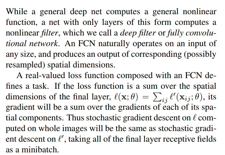
While a general deep net computes a general nonlinear function, a net with only layers of this form computes a nonlinear filter, which we call a deep filter or fully convolutional network. An FCN naturally operates on an input of any size, and produces an output of corresponding (possibly resampled) spatial dimensions.

This is a key distinction. A “general deep net” (one with fully connected layers) takes a fixed-size input and squashes it down to a single output vector. It’s a black box function. An FCN, on the other hand, acts like a sophisticated filter from signal processing. It slides over the input image, transforming it into an output map that preserves the spatial grid. This is why it can handle inputs of any size—the filter just has more area to slide over.

The Magic of the Loss Function

The next part is the most critical insight for understanding the efficiency of FCNs.

A real-valued loss function composed with an FCN defines a task. If the loss function is a sum over the spatial dimensions of the final layer, l(x; θ) = ∑_ij l’(x_ij; θ), its gradient will be a sum over the gradients of each of its spatial components. Thus stochastic gradient descent on l computed on whole images will be the same as stochastic gradient descent on l’, taking all of the final layer receptive fields as a minibatch.

This sounds complicated, but the idea is actually very intuitive. Let’s break it down.

1. “A loss function… defines a task.”: The loss function is what tells the network if its prediction is good or bad. For segmentation, the loss is typically calculated at every pixel. For example, for a pixel that is supposed to be “cat,” the network gets a high penalty (loss) if it predicts “dog.”

2. “The loss function is a sum over the spatial dimensions.”: To get the total loss for the entire image, you just add up the individual losses from every single pixel (or every location (i,j) in the final output map). The total image loss l is the sum of all the little pixel losses l'.

3. The “Aha!” Moment: Because of the rules of calculus (specifically, the sum rule of derivatives), the gradient of the total loss is simply the sum of the gradients from each individual pixel’s loss.

4. The Punchline: This means that performing one backpropagation step on the entire image is mathematically identical to performing many individual backpropagation steps on every single output pixel (or, more accurately, on every input patch that corresponds to an output pixel) and then averaging the gradients together.

In other words:

Training an FCN on one full image is the same as training a regular CNN on a giant batch of overlapping image patches taken from that image.

The FCN approach is just an incredibly efficient way to do this. Instead of running each patch through the network independently (which involves tons of redundant calculations on the overlapping parts), the FCN computes it all in one elegant, shared forward and backward pass.

The authors summarize this by saying it’s like taking all of the final layer’s receptive fields and treating them as a “minibatch”. This is the key insight that unlocks fast, efficient training for dense prediction tasks.

Laying Out the Plan

Having established the theoretical and efficiency benefits of the FCN paradigm, the authors now summarize the main point and provide a clear roadmap for the subsections that follow.

When these receptive fields overlap significantly, both feedforward computation and backpropagation are much more efficient when computed layer-by-layer over an entire image instead of independently patch-by-patch.

This sentence is the grand summary of the previous discussion. Because adjacent “patches” in an image overlap a great deal, processing them one by one is wasteful. An FCN exploits this overlap by sharing the computation, making both the forward pass (inference) and the backward pass (learning) vastly more efficient.

The Roadmap for FCN Design

The rest of the paragraph lays out the practical steps and design choices they will now explain in detail. It’s a preview of the rest of Section 3.

We next explain how to convert classification nets into fully convolutional nets that produce coarse output maps.

This is the first step: the “network surgery” we talked about. They will show how to take a network like VGG, chop off its final layers, and reinterpret the remaining layers as convolutions. The output will be a low-resolution or “coarse” map of predictions.

For pixelwise prediction, we need to connect these coarse outputs back to the pixels. Section 3.2 describes a trick that OverFeat [29] introduced for this purpose. We gain insight into this trick by reinterpreting it as an equivalent network modification.

Step two is dealing with the coarse output. How do you get a full-resolution prediction? They first analyze a previous method, the “shift-and-stitch” trick from the OverFeat paper. They promise to give a new perspective on how this trick actually works under the hood.

As an efficient, effective alternative, we introduce deconvolution layers for upsampling in Section 3.3.

This is where they introduce their preferred solution. Instead of a clever but potentially clunky trick like shift-and-stitch, they propose a more elegant, learnable, in-network solution: deconvolution layers. (Note: “deconvolution” is a slightly confusing term; today, this is more commonly called a “transposed convolution.” But the idea is the same: it’s a layer that upsamples its input.)

In Section 3.4 we consider training by patchwise sampling, and give evidence in Section 4.3 that our whole image training is faster and equally effective.

Finally, they will address the alternative training methodology head-on. They will analyze patchwise training and then, later in the paper, present experimental evidence that their whole-image training approach converges just as well (or better) and in a fraction of the time.

This paragraph effectively transitions us from the general theory of FCNs to the specific, practical details of their implementation. Let’s dive into these subsections one by one.

Summary of Section 3 (So Far): The Theory of FCNs

1. Fundamental Properties of Convnets: The section begins by establishing the basics.
   • Data in a CNN is a 3D volume (height x width x depth/channels).
   • The receptive field is a crucial concept: it’s the area of the original input that a neuron in a deeper layer is sensitive to. Receptive fields grow as you go deeper into the network.
   • The core operations (convolution, pooling) are built on translation invariance, meaning the same feature detector is applied everywhere. This makes them act like sliding filters.
2. Defining a Fully Convolutional Network (FCN):
   • A network composed only of these filter-like layers is called a “deep filter” or an FCN.
   • Crucially, unlike a traditional classifier with fixed-size layers, an FCN can naturally process an input of any size and will produce a corresponding spatial output map.
3. The Breakthrough in Training Efficiency: This is the most important insight of the section.
   • The total loss for a segmentation task is simply the sum of the individual losses at each pixel.
   • Because of this, the gradient calculation for the entire image is also just the sum of the gradients from each pixel.
   • This means that training an FCN on one whole image is mathematically equivalent to training a traditional CNN on a massive minibatch of overlapping image patches.
   • The FCN architecture is a computationally brilliant way to perform this batch training, sharing all the redundant computations and making the process incredibly fast and efficient.
4. The Road Ahead:
   • The section concludes by providing a roadmap for the rest of the technical discussion. The authors will now explain the practical steps:
     1. How to convert existing classification networks into FCNs.
     2. How to solve the problem of getting from the network’s coarse output map back to a full-resolution pixel prediction, first by analyzing an old method and then by proposing their superior alternative (deconvolution layers).
     3. Why their whole-image training approach is better than the common patch-based sampling method.

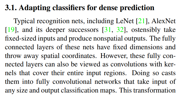
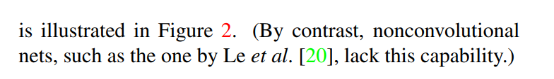
3.1. Adapting Classifiers for Dense Prediction

This section details the first and most fundamental trick in the FCN playbook: converting a standard image classification network into a network that can produce a spatial heatmap of predictions.

Let’s break this down, using the Figure 2 as our guide.

The Problem with Classifiers: Fully Connected Layers

As the text states, networks like AlexNet or VGG were designed for classification. They take an image (e.g., 224x224 pixels) and produce a “nonspatial output”—a simple list of 1000 scores, one for each possible class.

The reason they are locked into a fixed input size and lose all spatial information is because of their final layers, the fully connected (FC) layers.

• An FC layer connects every neuron from its input to every one of its output neurons.
• To do this, it first requires that its input is “flattened” into a fixed-length 1D vector. For example, a 7x7x512 feature map from the last convolutional layer is flattened into a single vector of 7 * 7 * 512 = 25,088 numbers.
• This flattening step is what “throws away spatial coordinates.” The network no longer knows what was next to what; it just has one long list of features.
• Because the weight matrix of the FC layer has a fixed size (e.g., 4096 outputs x 25,088 inputs), the input vector must always have a length of 25,088. This is why the original image had to be a fixed size.

The Solution: Viewing FC Layers as Convolutions

Here comes the key insight. The authors state that an FC layer can be perfectly mimicked by a convolutional layer. How?

Imagine that last 7x7x512 feature map. Instead of flattening it, let’s apply a convolutional layer where the kernel size is exactly 7x7. A 7x7 kernel will cover the entire 7x7 input feature map in one go. If this convolutional layer has 4096 output filters, it will produce a 1x1x4096 output map. This is mathematically identical to the 4096-element vector produced by the original FC layer!

This process of replacing FC layers with equivalent convolutional layers is what the paper calls “convolutionalization.”

The Magic of Convolutionalization (Figure 2)

Figure 2 illustrates this transformation beautifully.

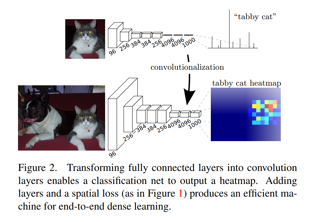
• The Top Path (Standard Classifier): A small, fixed-size image of a cat is fed into the network. After several convolutional/pooling layers, it’s processed by the FC layers to produce a single output vector, which correctly identifies the image as a “tabby cat.”

• The Bottom Path (The FCN): The network has been “convolutionalized.”

  1. Arbitrary-Sized Input: We can now feed it a larger image—one that contains both a dog and the cat. The convolutional parts of the network don’t mind; they just produce larger feature maps.
  2. Spatial Output (Heatmap): The layers that replaced the old FC layers now act like filters sliding over the larger feature map. The result is not a single 1x1 output, but a spatial grid of predictions—a “tabby cat heatmap.”
  3. Interpreting the Heatmap: The heatmap is hot in the region corresponding to the cat and cold elsewhere. The network is now telling us both what it sees (tabby cat) and where it sees it.

This simple reinterpretation is the key that unlocks the power of pre-trained classification networks for dense prediction tasks. It turns a tool designed to answer a single question (“What is in this image?”) into a tool that can answer a question for every location (“What is at this location?”).

Some questions?

Question 1: How can the FCN take a larger image?

We only changed the end of the network, so how does that affect what the beginning of the network can accept?

The key is to realize that the convolutional layers never had a fixed-size requirement in the first place. We were only pretending they did because the fully connected (FC) layer at the end forced our hand.

Let’s walk through the logic:

1. A Convolutional Layer is Flexible: Think about a single 3x3 convolution. It’s just a small filter that slides across its input. Does this filter care if it’s sliding over a 7x7 input or a 100x100 input? No. It will just slide more times on the bigger input and produce a bigger output map. The operation itself is independent of the input size. The same is true for pooling layers.

2. The Bottleneck was the FC Layer: The problem came at the transition from the last convolutional layer to the first FC layer. Let’s use AlexNet’s numbers.

   • The last convolutional layer (conv5) produces a feature map of size 6x6x256 (when the input is 227x227).
   • The first FC layer (fc6) expects its input to be a flattened vector of length 6 * 6 * 256 = 9216. This is a hard requirement. The weight matrix of this layer is fixed at size 4096 x 9216. It cannot accept a vector of any other length.

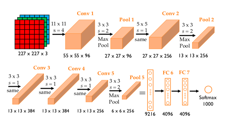
Image Source: Large-scale image recognition: AlexNet by Anh H. Reynolds

3. The Chain Reaction: Because fc6 demanded a 9216-element vector, conv5 had to produce a 6x6x256 map. For conv5 to produce a 6x6x256 map, its input had to be a certain size, and so on, all the way back to the very first layer. The fixed-size requirement of the final FC layer created a ripple effect backwards through the entire network, forcing the input image to be a fixed size (227x227).

4. Removing the Bottleneck: When we “convolutionalize” the network, we replace that rigid fc6 layer with a flexible convolutional layer. This new convolutional layer has a 6x6 kernel. It can slide over an input of any size. If the feature map from conv5 is 6x6, the new layer will produce a 1x1 output. If the feature map from conv5 is 10x10 (from a bigger input image), it will slide over it and produce a 5x5 output map.

In summary: The initial layers of the network were always capable of handling larger images. The only reason they were ever fed fixed-size inputs was to satisfy the rigid demands of the fully connected layer at the very end. By replacing that FC layer with a flexible convolution, we unleash the inherent flexibility of the entire network.

Question 2: What changed to make the last layer give a heatmap instead of “tabby cat”?

The output is still saying “tabby cat,” but it’s now saying it at every spatial location in its output grid.

Let’s trace the output:

1. Original Classifier Output: The very last FC layer in AlexNet (fc8) takes the 4096 features from the layer before it and outputs 1000 numbers. A softmax function is then applied to turn these numbers into probabilities. The highest probability (e.g., the 281st number, which corresponds to “tabby cat”) is the final prediction.

2. “Convolutionalized” Final Layer: We replace this final fc8 layer with a 1x1 convolutional layer that has 1000 output channels.

   • Input: It takes the output map from the previous layer (which might be, for example, a 5x5x4096 map).
   • Operation: A 1x1 convolution is very simple. At each of the 5x5 locations, it looks at the 4096 numbers (the feature vector for that location) and computes 1000 new numbers (the class scores for that location).
   • Output: The result is a 5x5x1000 output map.

3. Visualizing the Heatmap: This 5x5x1000 map is our final prediction. It’s a grid of class scores.

   • If we look at just one channel, say the 281st channel (the “tabby cat” channel), we get a 5x5 grid of numbers. These numbers represent the score for “tabby cat” at each of the 25 locations.
   • This 5x5 grid of scores is the heatmap. We can visualize it by coloring the locations with high scores red/yellow and locations with low scores blue.

In summary: We replaced the final layer that produced one list of 1000 class scores with a 1x1 convolution that produces a grid of 1000-score lists. The heatmap for a specific class (like “tabby cat”) is simply a visualization of that class’s score at every point in the output grid. The network is now effectively a sliding-window classifier, but one that runs extremely efficiently in a single forward pass.

Now that the authors have established how to turn a classifier into an FCN, they explain why this is such a good idea. The core concept here is amortized computation.

1. Equivalence and Amortization

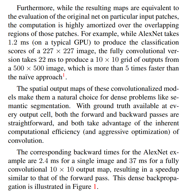
Furthermore, while the resulting maps are equivalent to the evaluation of the original net on particular input patches, the computation is highly amortized over the overlapping regions of those patches.

This is the key sentence. Let’s break it down:

• “equivalent to the evaluation… on particular input patches”: This means that if you take the final heatmap from the FCN, the prediction at a single point (i,j) is exactly the same as if you had cropped out the corresponding 227x227 patch from the original input image and fed it through the original classifier network. The results are identical.
• “computation is highly amortized”: “Amortized” is a term from accounting and computer science that means spreading a cost over many units. Here, the “cost” is the computational work of the convolutions. Instead of re-doing the work for every single patch (many of which overlap), the FCN does the computation just once. The cost is shared, or “amortized,” across all the patches.

2. Speedup by the Numbers

The authors then provide concrete numbers to show this isn’t just a theoretical benefit.

For example, while AlexNet takes 1.2 ms (on a typical GPU) to produce the classification scores of a 227 × 227 image, the fully convolutional version takes 22 ms to produce a 10 × 10 grid of outputs from a 500 × 500 image, which is more than 5 times faster than the naïve approach¹.

Let’s do the math on the “naïve approach”:

• The FCN produces a 10 x 10 = 100 grid of predictions.
• The naïve approach would be to run the original AlexNet on 100 different input patches.
• Time for naïve approach: 100 patches * 1.2 ms/patch = 120 ms.
• Time for FCN: 22 ms.
• Speedup: 120 ms / 22 ms ≈ 5.45 times faster.

This is a massive speedup, and it gets even bigger for larger images. This efficiency is what makes dense prediction with deep networks practical.

The naïve approach would be to run the original AlexNet on 100 different input patches

This describes the old, slow, “brute-force” way of doing semantic segmentation before FCNs.

Imagine you have a large 500x500 pixel image you want to segment. But the only tool you have is the original AlexNet, which is a classifier that only accepts small, fixed-size 227x227 images. How can you get a prediction for every pixel in your big image?

The “naïve approach” is to simulate a sliding window:

1. Crop a Patch: From your large 500x500 image, you would first crop a 227x227 patch from the top-left corner.
2. Classify It: You feed this single patch into AlexNet. The network processes it and gives you one prediction (e.g., “grass”). You assume this prediction applies to the center of the patch you just cropped.
3. Slide and Repeat: You then slide your cropping window a bit to the right (say, by 32 pixels), creating a new 227x227 patch that heavily overlaps with the first one. You feed this new patch into AlexNet and get another prediction.
4. Cover the Whole Image: You repeat this process, sliding the window across the entire 500x500 image, until you have a prediction for every location. To get the 10x10 grid of predictions mentioned in the paper, you would have to do this 10 * 10 = 100 times.

Why is this “naïve”? It is incredibly wasteful. The second patch you process shares about 85% of its pixels with the first patch. But the naïve approach runs the entire AlexNet computation from scratch for both patches. All the work done on the overlapping pixels is thrown away and re-computed again and again.

The FCN, by processing the whole image at once, performs this computation for each pixel exactly once and shares the results—this is the “amortization” they talk about.

3. A Natural Fit for Dense Learning

The spatial output maps of these convolutionalized models make them a natural choice for dense problems like semantic segmentation. With ground truth available at every output cell, both the forward and backward passes are straightforward, and both take advantage of the inherent computational efficiency…

The authors are saying that this architecture isn’t just a clever hack; it’s a perfect match for the problem. Since the network outputs a spatial map, we can directly compare it to our ground truth segmentation map (which is also a spatial map). We can define a loss at every single “output cell” or pixel.

And because of the efficiency they just described, the backward pass (backpropagation) for learning is also incredibly fast.

4. Fast Learning, Too

The corresponding backward times for the AlexNet example are 2.4 ms for a single image and 37 ms for a fully convolutional 10 × 10 output map, resulting in a speedup similar to that of the forward pass. This dense backpropagation is illustrated in Figure 1.

Just as the forward pass is faster, the backward pass benefits from the same amortization. Learning on one large image is much faster than learning on 100 individual patches. This is a crucial point: the FCN architecture speeds up not just inference (making predictions) but also training (learning the weights).

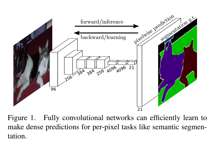
Figure 1 in the paper visually represents this idea: the data flows forward through the whole image to produce a dense prediction map, and the error signals flow backward through the whole image to update the weights. It’s a single, efficient, end-to-end process.

Let’s break down this crucial paragraph.

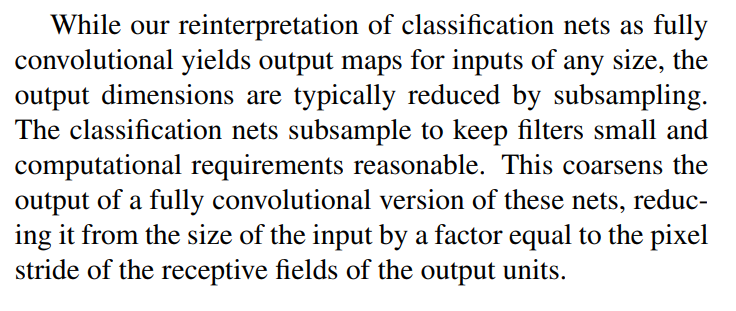
1. The Cause: Subsampling

The problem is subsampling (also known as downsampling). Inside any deep classification network like VGG, there are pooling layers (e.g., max pooling) or convolutions with a stride greater than 1.

• Why do they subsample? The paragraph gives two reasons:
  1. To keep filters small: Subsampling allows the network to increase the receptive field of its filters without increasing the kernel size. A 3x3 filter after a 2x pooling layer “sees” a larger area of the original image than a 3x3 filter with no pooling. This allows the network to learn about larger structures efficiently.
  2. To keep computational requirements reasonable: Each time you subsample, you dramatically reduce the size of the feature map (e.g., a 2x2 max pool cuts the number of activations by 75%). This saves a huge amount of memory and computation in the deeper layers.

2. The Effect: Coarse Output

While subsampling is essential for efficient classification, it has a major downside for segmentation: it “coarsens” the output.

• Imagine a 224x224 input image.
• A network like VGG might have a total of five 2x pooling layers.
• The total subsampling factor is 2 * 2 * 2 * 2 * 2 = 32.
• This means the final feature map before the classifier will be 224 / 32 = 7, so it’s a 7x7 grid.
• Our FCN’s output heatmap will therefore also be a 7x7 grid.

A 7x7 prediction is extremely coarse! Each cell in that grid corresponds to a large 32x32 block of pixels in the original input. This is the “What vs. Where” problem in action. We might know that one of these 32x32 blocks contains a cat, but we have lost all the fine-grained detail needed to draw the cat’s exact outline.

3. The “Pixel Stride”

The authors formalize this by saying the output is reduced by a factor equal to the “pixel stride of the receptive fields of the output units.” This is a more technical way of saying the same thing. The “pixel stride” is just the total subsampling factor. It describes how far apart the centers of the receptive fields of adjacent output units are in the original pixel space. If the total stride is 32, it means one output cell is looking at a patch of the input, and the very next output cell is looking at a patch whose center is 32 pixels away.

This perfectly sets the stage for the next sections, which will explore different strategies for taking this coarse heatmap and turning it into a dense, pixel-perfect segmentation.

3.2. Shift-and-stitch is filter rarefaction

We’ve established the problem: our FCN produces a coarse output map because of subsampling. For example, if the network has a total stride of f=2, the output map is half the size of the input. We only have a prediction for every other pixel. How do we fill in the gaps?

This section analyzes one of the first proposed solutions, a trick from the OverFeat paper called “shift-and-stitch”.

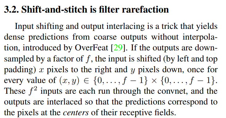
This sounds very complex, so let’s break it down with a simple example.

The “Shift-and-Stitch” Trick Explained

Imagine our network has a total subsampling factor of f=2. This means our output is half the height and half the width of the input. We are “missing” the predictions for many pixels.

The shift-and-stitch trick says we can get these missing predictions by re-running the network multiple times on slightly shifted versions of the input image.

Let’s say f=2. The number of runs we need is f² = 2² = 4. The shifts (x, y) will be: (0,0), (0,1), (1,0), and (1,1).

1. Run 1: Shift (0,0) - No shift.
   • We feed the original image into our FCN.
   • It produces a coarse output map. These are our predictions for a grid of pixels (0,0), (0,2), (0,4)..., (2,0), (2,2), (2,4)..., etc.
2. Run 2: Shift (0,1) - Shift down by 1 pixel.
   • We take the original image and shift the whole thing down by one pixel (padding the top with zeros).
   • We feed this new, shifted image into the FCN.
   • Because the input was shifted, the output predictions now correspond to a different grid of pixels in the original image space: (1,0), (1,2), (1,4)..., (3,0), (3,2), (3,4)..., etc.
3. Run 3: Shift (1,0) - Shift right by 1 pixel.
   • We shift the original image to the right by one pixel.
   • The FCN’s output now corresponds to the grid (0,1), (0,3), (0,5)..., (2,1), (2,3), (2,5)..., etc.
4. Run 4: Shift (1,1) - Shift right by 1 and down by 1.
   • We shift the image both right and down.
   • The FCN’s output now corresponds to the final missing grid: (1,1), (1,3), (1,5)..., (3,1), (3,3), (3,5)..., etc.

The “Stitch” Part: After these four runs, we have four different coarse output maps. The “stitch” (or “interlace”) part is simple: we weave them together. We take the first prediction from the first map, the first from the second, the first from the third, and so on, to build a new, dense output map that is f times larger and contains predictions for every single pixel.

The Downside: This trick works, but it’s inefficient. We had to run our network f² times (in this case, 4 times) just to get one dense prediction. The authors of FCN are looking for a way to get the same result, but with the efficiency of a single pass. Their analysis in the rest of this section will show how.

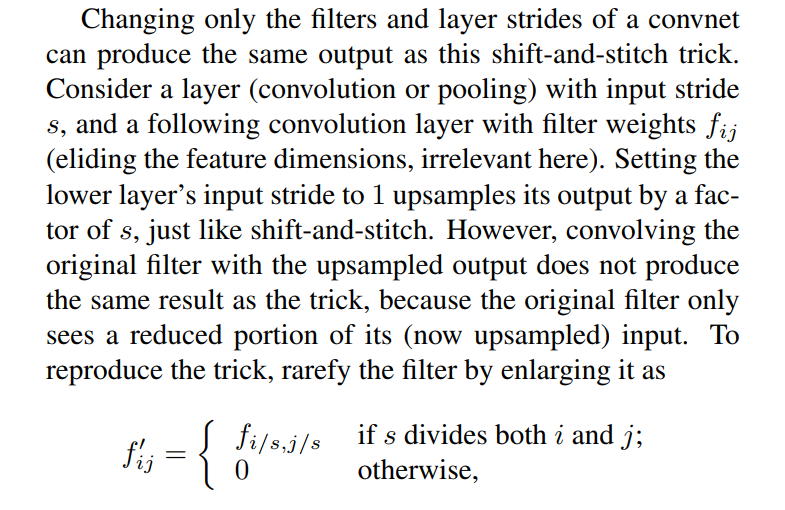
The authors start with a bold claim:

Changing only the filters and layer strides of a convnet can produce the same output as this shift-and-stitch trick.

Instead of running the network f² times on shifted inputs, they are saying you can modify the network itself to get the exact same dense output in a single pass. How?

Let’s follow their logic.

Step 1: Remove the Subsampling

Consider a layer (convolution or pooling) with input stride s… Setting the lower layer’s input stride to 1 upsamples its output by a factor of s…

Let’s say we have a pooling layer with a stride s=2. This is what causes the subsampling. The most obvious way to prevent subsampling is to simply change the stride to s=1. Now, the output feature map from this layer will be the same size as its input. We have successfully produced a denser output.

Step 2: The Problem with Step 1

But wait, it’s not that simple.

However, convolving the original filter with the upsampled output does not produce the same result as the trick, because the original filter only sees a reduced portion of its (now upsampled) input.

This is the crucial problem. Let’s say the next layer has a 3x3 filter.

• Original Network (with stride 2): The 3x3 filter looks at a 3x3 patch of the coarse feature map. Because that map was subsampled by a factor of 2, this 3x3 patch corresponds to a larger region of the original input. The filter has a large receptive field.
• Modified Network (stride set to 1): We removed the subsampling. Now the 3x3 filter looks at a 3x3 patch of a dense feature map. It is now looking at a much smaller, finer-grained region of the original input. We have shrunk its receptive field!

By naively changing the stride to 1, we made the output denser, but we broke the network. The filters in the deeper layers are no longer seeing the world the way they were trained to; their view has become narrow and myopic.

Step 3: The Solution - “Filter Rarefaction”

How do we give the filter its wide view back? The answer is to “rarefy” the filter. “Rarefy” means to make something less dense. In this context, it means we are going to enlarge the filter by inserting holes (zeros) into it. This is also known as an atrous convolution or dilated convolution.

To reproduce the trick, rarefy the filter by enlarging it as f’_ij = { f_{i/s, j/s} if s divides both i and j; 0 otherwise }

Let’s translate this equation with our s=2 example. Imagine our original 3x3 filter f looks like this:

[w1, w2, w3]
[w4, w5, w6]
[w7, w8, w9]

To “rarefy” it, we create a new, larger filter f' by taking the original weights and spreading them out, filling the gaps with zeros. For s=2, we put a zero between each original weight. The new rarefied 5x5 filter f' would look like this:

[w1,  0, w2,  0, w3]
[ 0,  0,  0,  0,  0]
[w4,  0, w5,  0, w6]
[ 0,  0,  0,  0,  0]
[w7,  0, w8,  0, w9]

This new, larger, “holey” filter now operates on the dense feature map (the one we got by setting the stride to 1). Because the filter is spread out, it now sees the exact same large receptive field as the original 3x3 filter did on the coarse map.

The Punchline: By applying this process—(1) setting the stride of a pooling layer to 1, and (2) rarefying the filter of the next convolutional layer—we have perfectly reproduced the result of the complex shift-and-stitch trick, but we can do it all in a single, efficient forward pass. This is a profound insight that would later lead to the popularization of dilated convolutions in segmentation models like DeepLab.

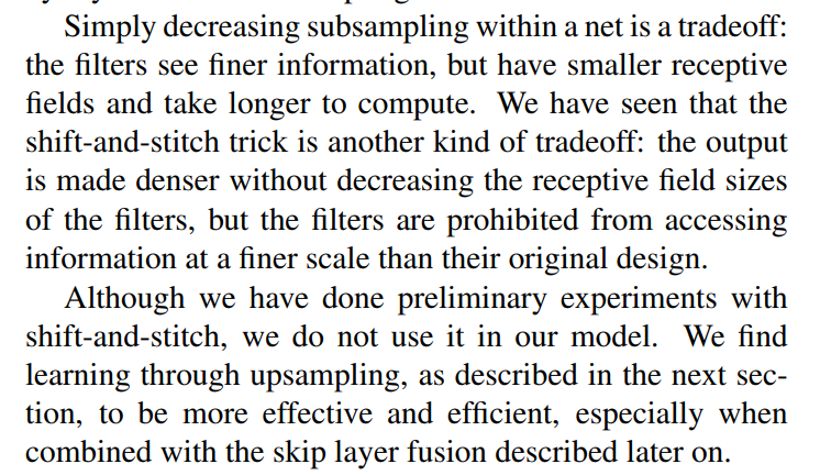
After deconstructing the “shift-and-stitch” trick and showing its equivalence to modifying the network’s filters (“filter rarefaction” or dilated convolution), the authors now step back to evaluate the tradeoffs and explain why they are ultimately going to choose a different path.

Two Kinds of Tradeoffs

The authors identify two distinct ways to get denser predictions, each with its own pros and cons.

1. The Simple Way: “Decreasing subsampling”

   Simply decreasing subsampling within a net is a tradeoff: the filters see finer information, but have smaller receptive fields and take longer to compute. This refers to the naive approach we discussed: just setting the stride of a pooling layer to 1.

   • Pro: The filters now operate on a dense map, so they can see very fine-grained details.
   • Con 1 (Smaller Receptive Fields): As we saw, this shrinks the effective receptive field of deeper layers, preventing them from seeing the “big picture.” The network loses crucial context.
   • Con 2 (Slower): Processing dense feature maps through the entire network is computationally very expensive.

2. The Clever Way: “Shift-and-stitch” / Filter Rarefaction

   We have seen that the shift-and-stitch trick is another kind of tradeoff: the output is made denser without decreasing the receptive field sizes of the filters, but the filters are prohibited from accessing information at a finer scale than their original design. This refers to the method they just analyzed.

   • Pro: It cleverly makes the output dense while preserving the large receptive fields of the original network design. This is a big win.
   • Con: The “holey” or rarefied filters systematically skip information. The filter [w1, 0, w2, 0, w3] will never see the information from the pixels that land on the zeros. It’s locked into looking at the world with a specific, coarse grid. It is “prohibited from accessing information at a finer scale.” It can’t see the fine details that the “simple way” could.

The Verdict: A Better Way Forward

Having analyzed these two options, the authors declare their choice.

Although we have done preliminary experiments with shift-and-stitch, we do not use it in our model. We find learning through upsampling, as described in the next section, to be more effective and efficient, especially when combined with the skip layer fusion described later on.

This is a critical pivot. They acknowledge the cleverness of shift-and-stitch/filter rarefaction but ultimately reject it. They have found a third option that they believe is superior:

1. Keep the original network as is: Let the network do its subsampling and produce a coarse, low-resolution but semantically rich feature map.
2. Learn to upsample: Then, add new layers to the end of the network whose job is to intelligently upsample this coarse map back to the full resolution.
3. Fuse with skip layers: They also tease their most important architectural innovation: they will combine this upsampling process with “skip connections” that bring in fine-detail information from the shallow layers.

This sets the stage perfectly for Section 3.3, where they will introduce their chosen upsampling method: the “deconvolution” or transposed convolution layer.

3.3. Upsampling is backwards strided convolution

We have a coarse, low-resolution prediction map from our network. How do we get back to a dense, full-resolution prediction? The authors propose a new, elegant, and learnable approach.

They begin by introducing the general concept using a familiar idea: interpolation.

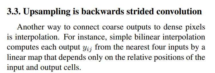
The Simple Idea: Interpolation

Imagine you have a tiny 2x2 image and you want to make it 4x4. How do you fill in all the new pixels?

Bilinear interpolation is a standard method to do this. For each new pixel you want to create, you look at the 4 closest pixels in the original coarse image. You then calculate the new pixel’s value as a weighted average of those 4 neighbors. The closer a neighbor is, the more weight it gets in the average.

This is a fixed, mathematical procedure. It’s a simple “linear map” that smoothly blends the existing values to fill in the gaps. It’s a reasonable starting point, but it’s not very intelligent. It will always produce a somewhat blurry result because it’s just averaging.

The Big Idea: Learnable Upsampling

The authors’ key insight is that since interpolation can be expressed as a linear operation, it can be implemented within the network itself. And if it’s in the network, it can be learned.

This leads them to the core idea of this section: backwards strided convolution, which is also commonly known as transposed convolution or, somewhat misleadingly, deconvolution.

Let’s think about what a normal convolution with a stride does:

• Normal Strided Convolution (Downsampling): It’s a many-to-one mapping. It takes a patch of input values (e.g., a 3x3 patch) and computes a single output value. If the stride is greater than 1, the output map is smaller than the input map. It reduces resolution.

A backwards strided convolution does the exact opposite:

• Backwards Strided Convolution (Upsampling): It’s a one-to-many mapping. It takes a single input value from the coarse map and projects it onto a patch of the larger output map. It effectively “splats” or “paints” the input value onto a larger grid, increasing the resolution. The weights of the filter control the shape and values of this “splat.”

This operation is called a “backwards” convolution because it uses the same connectivity pattern as a regular convolution, but in the reverse direction (from output to input). It’s the operation needed to compute the gradients in the backward pass of a normal convolution, which is why it’s a natural fit for deep learning libraries.

Formalizing Upsampling as a Convolution

The authors now provide the formal connection between upsampling and convolution.

This is a very elegant way to think about it.

• A normal convolution with a stride of s=2 skips every other input pixel.
• An upsampling operation with a factor of f=2 could be thought of as a convolution with a stride of s=1/2, meaning it processes “in-between” pixels that don’t yet exist.
• While a “fractional stride” is just a conceptual device, it leads to a concrete implementation: the backwards convolution (or transposed convolution). This layer does exactly what’s needed. It takes a coarse input and produces a dense output, with the upsampling factor controlled by its stride.
• The final sentence highlights why this was a practical choice: deep learning frameworks (like Caffe, which they used) already had this operation built-in, because it’s the same operation needed to compute gradients for a regular convolution. So, implementing it was easy.

The Power of Learnable Upsampling

This is the punchline of the whole section. Why is this approach better than just using a fixed function like bilinear interpolation?

This is the critical advantage.

1. End-to-end Learning: Because the upsampling is just another layer in the network, it can be trained along with all the other layers. The error signal from the final pixelwise loss flows all the way back through the deconvolution layers, teaching them how to upsample better.
2. It can be Learned: The weights of the deconvolution filter are not fixed. The network can learn the optimal way to go from a coarse to a fine representation for the specific task. For example, it might learn that when it sees a coarse blob for “car,” the best way to upsample it is to create sharp, straight lines at the edges. A fixed bilinear filter could never learn this; it would just create a blurry blob.
3. Nonlinear Upsampling: By stacking multiple deconvolution layers with activation functions (like ReLU) in between, the network can learn an even more powerful, nonlinear mapping from the coarse space to the dense space.

The Authors’ Final Choice

In our experiments, we find that in-network upsampling is fast and effective for learning dense prediction. Our best segmentation architecture uses these layers to learn to upsample for refined prediction in Section 4.2.

The authors conclude the section by stating their verdict. This method of using learnable deconvolution/transposed convolution layers is their chosen weapon for tackling the coarse output problem. It’s efficient, it’s powerful because it’s learnable, and it fits perfectly into their end-to-end training philosophy.

Summary of Sections 3.1-3.3: From Coarse Classifiers to Dense Predictors

Section 3.1: The Core Idea and Its Flaw

• The Idea: “Convolutionalization”. We can take a powerful, pre-trained image classifier (like VGG or AlexNet) and make it produce a spatial prediction map. We do this by replacing the final, rigid fully connected layers with equivalent convolutional layers.
• The Benefits: This simple trick makes the network flexible (it can accept inputs of any size) and incredibly efficient. A single pass over a large image is mathematically equivalent to, but much faster than, running the original classifier on thousands of overlapping patches. This applies to both inference and training.
• The Flaw: Coarse Output. The resulting prediction map is very low-resolution. Because of repeated subsampling (pooling layers) in the original network, the output might have a stride of 32, meaning one prediction covers a large 32x32 block of input pixels. This is too “blurry” for precise segmentation.

Section 3.2: Analyzing a Prior Solution (And Rejecting It)

• The Problem: How do we get from the coarse map to a dense, pixel-perfect one?
• An Existing Trick: “Shift-and-Stitch”. One method (from the OverFeat paper) involves running the network multiple times on slightly shifted versions of the input and then weaving the results together. This is clever but inefficient.
• A Deeper Insight: “Filter Rarefaction”. The authors show that the shift-and-stitch trick is mathematically equivalent to a network modification: removing the subsampling (by setting layer strides to 1) and making the convolutional filters “holey” to preserve their receptive fields (also known as dilated/atrous convolution).
• The Verdict: While this method preserves context (large receptive fields), the “holey” filters systematically skip pixels and are prevented from seeing fine-grained information. The authors conclude it’s a clever but flawed tradeoff and look for a better way.

Section 3.3: The FCN’s Chosen Solution

• The New Idea: In-Network Upsampling. Instead of avoiding subsampling, the FCN approach embraces it. Let the network produce a coarse, semantically rich feature map, and then learn how to upsample it.
• The Mechanism: “Backwards Convolution”. The authors propose using transposed convolution (which they call “backwards convolution” or “deconvolution”) as the upsampling layer. This operation is a natural inverse to a standard convolution and was already available in deep learning frameworks.
• The Killer Feature: It’s Learnable. Crucially, the upsampling filter is not fixed (like traditional bilinear interpolation). Its weights are learned during end-to-end training. The network itself learns the best way to create a high-resolution prediction from a low-resolution feature map. It can even be stacked to learn powerful, nonlinear upsampling.
• The Conclusion: This method is fast, effective, and fits perfectly into the end-to-end learning paradigm. It becomes the foundational building block for the final FCN architecture.

4. Segmentation Architecture

Having established the theoretical components—convolutionalization, the coarse output problem, and learnable upsampling—the authors now detail how they assemble these parts into a state-of-the-art segmentation architecture. This section is the practical “recipe.”

They begin with a high-level overview of their entire process, followed by the specific details of their experimental setup.

The Overall Strategy

This first paragraph is a perfect summary of their entire architectural contribution. It’s a three-step plan:

1. Adapt: Take a pre-trained classifier (“ILSVRC classifier”) and “cast” it into an FCN using the convolutionalization trick from Section 3.1.
2. Upsample: Augment this base FCN with the in-network upsampling layers (transposed convolutions from Section 3.3) to learn how to produce dense predictions. The network is trained end-to-end with a “pixelwise loss.”
3. Refine: Create a “novel skip architecture.” This is the final and most important piece. They will build connections that “skip” over parts of the network to combine the deep, “coarse, semantic” information (the “what”) with the shallow, “local, appearance” information (the “where”). This is the key to getting predictions that are both accurate and detailed.

The Proving Grounds: Dataset and Metrics

Before showing their results, the authors define the rules of the game: the dataset they’re using, how the model learns, and how its performance is measured.

Let’s break down these critical experimental details:

• The Dataset: PASCAL VOC 2011. This was one of the premier, most challenging benchmarks for computer vision at the time. Proving your model’s worth on this dataset was a big deal.

• The Loss Function: “per-pixel multinomial logistic loss.” This is a fancy name for a simple idea. It’s the standard cross-entropy loss used for classification, but applied independently at every single pixel.

  • For each pixel, the network outputs a set of scores for all possible classes (e.g., cat, dog, sky, background).
  • The loss function compares this prediction to the one-hot encoded ground truth label for that pixel.
  • The total loss for the image is just the average of the losses over all pixels.

• The Evaluation Metric: “mean pixel intersection over union (mIoU).” This is the gold standard for evaluating segmentation quality. It’s much more telling than simple pixel accuracy.

  • For a single class (e.g., “car”), the IoU is calculated as: IoU = (Area of Overlap) / (Area of Union)
  • Area of Overlap (Intersection): The number of pixels that were correctly predicted as “car.”
  • Area of Union: The total number of pixels that were labeled as “car” in either the prediction OR the ground truth.
  • IoU is a strict metric. It punishes both false positives (predicting “car” where there isn’t one) and false negatives (failing to predict a “car” where there is one).
  • Mean IoU (mIoU): The IoU is calculated for every class, and then the scores are averaged. This gives a single, robust number that represents the model’s overall performance.

• Handling Ambiguity: The training “ignores pixels that are masked out.” This is standard practice. Datasets often have ambiguous regions (e.g., a blurry boundary) that are excluded from the loss calculation so the model isn’t penalized for a problem that even human labelers couldn’t solve.

4.1. From Classifier to Dense FCN

In this section, the authors execute the first part of their plan: take off-the-shelf classifiers, turn them into FCNs, and see how well they perform on segmentation “out of the box” after fine-tuning. This serves as a crucial baseline to measure all future improvements against.

The Process: A Step-by-Step Recipe

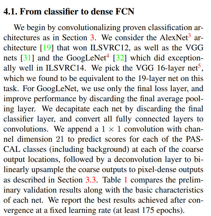
This is the concrete recipe for creating their simplest FCN, which they will later call FCN-32s.

1. Choose a Backbone: They start with three of the most famous and powerful classification networks of the era: AlexNet, VGG16, and GoogLeNet.
2. “Decapitate”: They perform the network surgery from Section 3.1. They chop off the final classification layer (which was specific to the 1000 ImageNet classes) and convert all the fully connected layers into equivalent convolution layers.
3. Add a Prediction Head: They need the network to predict scores for the PASCAL VOC classes, not the ImageNet ones. So, they add a new 1x1 convolution layer at the very end. The number of output channels is 21 (20 object classes in PASCAL + 1 for the background). This 1x1 convolution is what produces the final, coarse prediction map.
4. Upsample: To get a final prediction, they need to get from the coarse map back to the original image size. For this first simple baseline, they use a single deconvolution (transposed convolution) layer that performs a fixed bilinear upsampling. They are not using learnable upsampling or skip connections yet. This is the simplest possible way to get a dense output.

The Results: VGG is the Clear Winner (Table 1)

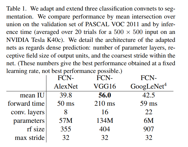
Let’s interpret these results:

• Accuracy (mean IU): FCN-VGG16 is the undisputed champion, scoring 56.0 mIoU. This is a huge leap over both AlexNet (39.8) and GoogLeNet (42.5). This demonstrates that the quality of the pre-trained features from the backbone network is critically important. VGG’s simple, deep, and uniform architecture seems to produce features that are more transferable to the segmentation task.
• Speed (forward time): FCN-VGG16 is by far the slowest at 210 ms. This is the price of its depth and large number of parameters. AlexNet and GoogLeNet are much faster, at 50-60 ms.
• Size (parameters): VGG is a beast, with 134 million parameters. AlexNet is also large (57M). GoogLeNet is famously efficient, achieving good classification performance with only 6M parameters, but this efficiency doesn’t seem to translate into top-tier segmentation performance in this simple FCN setup.
• Architecture (layers, rf size, stride): We can see that VGG is much deeper than AlexNet. All three networks have a maximum stride of 32, which confirms that their output before upsampling is very coarse (1/32nd of the input size).

The key takeaway from this section is: Even this simple “decapitate and upsample” approach, when applied to a strong backbone like VGG16, can produce very respectable segmentation results. The next step is to see how much better they can do by getting more sophisticated.

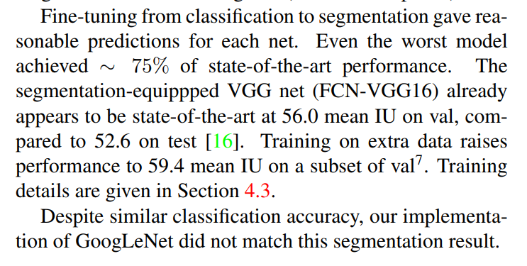
Let’s unpack these important claims:

1. Transfer learning works: The fact that simply fine-tuning pre-trained classifiers gives “reasonable predictions” is a major validation of their core approach. Even their FCN-AlexNet, the worst of the three, is still in the ballpark of the best prior methods.
2. The baseline FCN is already state-of-the-art: This is a huge result. Their FCN-VGG16, which is the most basic version of their architecture (later called FCN-32s), scores 56.0 mIoU on the validation set. This is already better than the 52.6 mIoU achieved on the test set by the previous state-of-the-art model, SDS [16]. SDS was a much more complex, multi-stage pipeline involving region proposals and post-processing. The fact that a simple, end-to-end FCN can beat it is a powerful statement about the elegance and effectiveness of their method.
3. More data helps: They mention that when they train on a larger dataset (the one used by the SDS authors), their score improves even further to 59.4 mIoU. This is a standard finding in deep learning, but it confirms their model benefits from more data.

The GoogLeNet Anomaly

Finally, they comment on a slightly puzzling result from their experiments.

Despite similar classification accuracy, our implementation of GoogLeNet did not match this segmentation result.

This is an interesting aside. On the original ImageNet classification task, VGG16 and GoogLeNet had very similar top-tier performance. You might expect, therefore, that they would also perform similarly on segmentation when used as backbones. But they don’t; FCN-VGG16 is much better.

The authors don’t give a definitive reason, but this finding suggests that raw classification accuracy isn’t the only thing that matters for transfer learning. The internal feature representations of the network matter a great deal. It seems that VGG’s simpler, more uniform structure with its large, feature-rich convolutional layers produces representations that are more readily adapted for the dense, spatial task of segmentation than GoogLeNet’s more complex “Inception” modules.

With these strong baseline results in hand, the authors have set the stage perfectly. They have shown that even their simplest model is a state-of-the-art contender. Now, in Section 4.2, they will introduce the “skip architecture” to show how they can improve upon this already impressive result.

4.2. Combining what and where

The previous section showed that a simple FCN (which they will call FCN-32s) can achieve state-of-the-art results. But the authors aren’t satisfied. They know the output is still crude. Now, they will introduce their novel architecture to fix this.

Restating the Problem: Coarse Outputs

They begin by reminding us of the core problem.

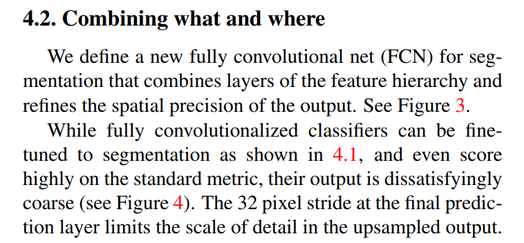
This paragraph sets the stage perfectly.

• The Goal: To create a new FCN architecture that “refines the spatial precision of the output.”
• The Motivation: The baseline FCN-32s model, despite its high mIoU score, produces visually unappealing, “blobby” segmentations. You can see this clearly in the first column of Figure 4. The mIoU metric rewards getting the general location of objects correct, but it doesn’t heavily penalize fuzzy boundaries.
• The Cause: The root cause is the 32 pixel stride. The final prediction is made from a feature map that is 1/32nd the resolution of the input. When you upsample this tiny map by a factor of 32, you are forced to make the same prediction for large blocks of pixels, which washes out all the fine details.

The problem is clear: the final prediction layer has great semantic information (it knows what it’s looking at) but terrible spatial information (it has no idea where the precise boundaries are). How can we re-introduce that missing spatial information? The answer is the skip architecture.

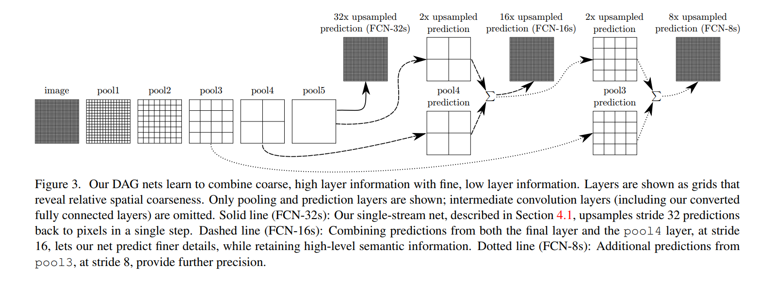
The caption calls this a “DAG net”. DAG stands for Directed Acyclic Graph. This is a departure from a standard classification network, which has a simple linear topology (layer 1 -> layer 2 -> layer 3…). Here, the information flows along multiple paths and gets combined, creating a graph-like structure.

The diagram shows how three different versions of the FCN are constructed.

1. FCN-32s (Solid Line) - The Baseline

• Path: This follows the solid black arrow. The network processes the image through all its pooling layers (pool1 through pool5) until it reaches the final, deepest, and most coarse layer. This layer has a stride of 32 relative to the input.
• Prediction: A prediction is made from this pool5 layer.
• Upsampling: This coarse prediction is then upsampled by a factor of 32 in a single giant step to get back to the original image resolution.
• Analysis: This is the simple baseline model from Section 4.1. It relies entirely on the deep semantic information from the last layer. As we know, this results in coarse, “blobby” segmentations.

2. FCN-16s (Dashed Line) - The First Refinement

This is the first and most important step in the skip architecture.

• The Problem: The FCN-32s prediction is too coarse.
• The Idea: Let’s get some spatial detail from an earlier, less coarse layer. The authors choose pool4, which has a stride of 16.
• The Architecture:
  1. First, the pool5 prediction is upsampled by a factor of 2x (using a transposed convolution). Now it has the same dimensions as the pool4 layer.
  2. A prediction is also made directly from the pool4 layer (by adding a 1x1 convolution head). This prediction is spatially finer but semantically weaker than the pool5 prediction.
  3. Fuse: The two predictions (the upsampled pool5 one and the pool4 one) are combined, typically by element-wise addition (indicated by the ∑ symbol).
  4. Final Upsampling: This new, fused prediction map, which is at a stride of 16, is then upsampled by a factor of 16 to get the final full-resolution output.
• Analysis: This is the core of the “what meets where” idea. The upsampled pool5 prediction provides the strong semantic guidance (the “what”), while the pool4 prediction provides more precise spatial details (the “where”). By fusing them, the network can learn to correct the coarse pool5 predictions using the finer information from pool4.

3. FCN-8s (Dotted Line) - The Second Refinement

This is just a logical extension of the FCN-16s idea.

• The Problem: FCN-16s is better, but maybe we can make it even more precise.
• The Idea: Let’s add even finer-grained detail from an even earlier layer, pool3, which has a stride of 8.
• The Architecture:
  1. Take the fused 16s prediction map (the one we got by combining pool5 and pool4).
  2. Upsample this map by a factor of 2x. Now it has the same dimensions as the pool3 layer.
  3. Make a new prediction directly from the pool3 layer.
  4. Fuse: Combine the upsampled 16s map with the new pool3 prediction.
  5. Final Upsampling: This final fused map, now at a stride of 8, is upsampled by a factor of 8 to get the final output.
• Analysis: This architecture creates a cascade of refinements. The pool5 prediction is refined by pool4, and that result is further refined by pool3. Each skip connection adds another level of detail to the final prediction.

In summary, Figure 3 shows a systematic way to solve the coarse prediction problem. Instead of a single, massive upsampling leap (32x), the FCN-16s and FCN-8s models use a series of smaller upsampling steps, injecting high-resolution feature information at each stage to progressively refine the segmentation boundaries.

This paragraph explains the philosophy behind the skip architecture.

• It’s a DAG (Directed Acyclic Graph), not a simple line.
• “Local predictions that respect global structure”: This is the perfect summary of the goal. The prediction from a shallow layer (pool4) is “local” (spatially precise), but it lacks context. The prediction from the deep layer (pool5/conv7) provides the “global structure” (the semantic understanding). The skip connection fuses them to get the best of both worlds.
• “Deep Jet”: This is the cool name they give to their architecture, drawing an analogy to a classic concept in computer vision scale-space theory.

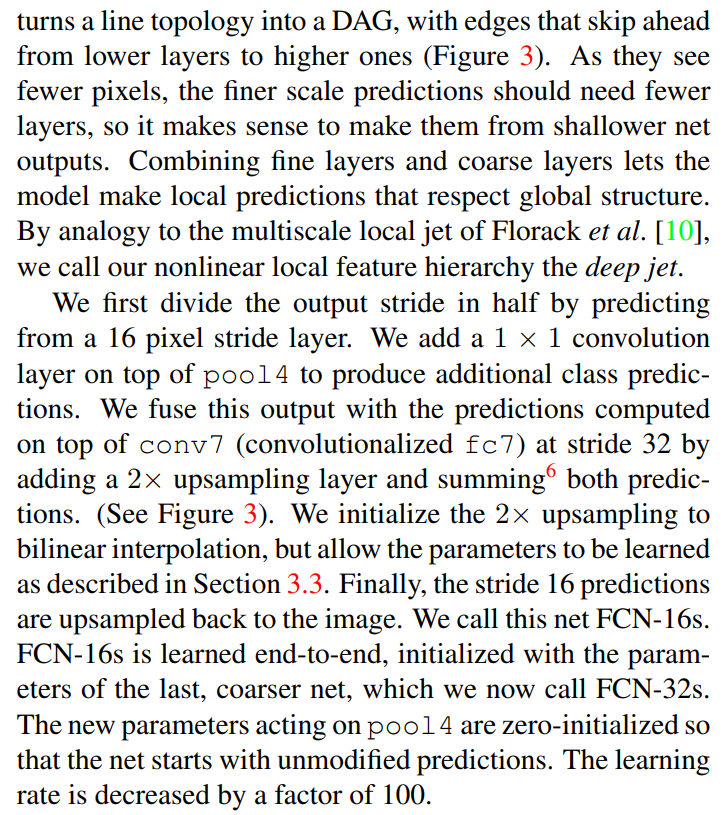
The Concrete Recipe for FCN-16s

The next part is the step-by-step implementation guide for the FCN-16s model.

We first divide the output stride in half by predicting from a 16 pixel stride layer. We add a 1 × 1 convolution layer on top of pool4 to produce additional class predictions. We fuse this output with the predictions computed on top of conv7 (convolutionalized fc7) at stride 32 by adding a 2× upsampling layer and summing both predictions. (See Figure 3). We initialize the 2× upsampling to bilinear interpolation, but allow the parameters to be learned… Finally, the stride 16 predictions are upsampled back to the image. We call this net FCN-16s.

This exactly matches the “dashed line” path we traced in Figure 3:

1. Take the final stride-32 prediction from conv7.
2. Upsample it by 2x using a learnable transposed convolution. (They note they initialize this layer’s weights to perform simple bilinear upsampling, which is a common and effective trick to give the training a good starting point).
3. Take the pool4 feature map (which is at stride 16).
4. Add a new 1x1 convolution layer on top of pool4 to make a class prediction at this finer scale.
5. Fuse: Add the results of step 2 and step 4 together.
6. Take the fused map and upsample it by 16x to get the final, full-resolution output.

The Training Strategy: Staged Fine-tuning

The final part is a crucial detail about how they train this more complex model. They don’t train it from scratch.

FCN-16s is learned end-to-end, initialized with the parameters of the last, coarser net, which we now call FCN-32s. The new parameters acting on pool4 are zero-initialized so that the net starts with unmodified predictions. The learning rate is decreased by a factor of 100.

This is a very clever, staged training approach:

1. First, train FCN-32s: They take their simple baseline model and train it until it converges.
2. Initialize FCN-16s: They build the FCN-16s architecture and initialize its weights using the already-trained weights from the FCN-32s model. The “backbone” of the network is already good to go.
3. Zero-initialize the new parts: What about the brand new 1x1 convolution layer they added on top of pool4? They zero-initialize it. This is a brilliant trick. If the weights of this new layer are all zero, then at the very beginning of training, it adds nothing to the fused prediction. This means that at iteration zero, the FCN-16s model produces the exact same output as the FCN-32s model it was initialized from. The network starts from a known, good state.
4. Fine-tune with a low learning rate: They then continue training (fine-tuning) the whole FCN-16s network end-to-end, but with a much smaller learning rate. This allows the network to gently learn how to use the new pool4 information to refine the already-good predictions from the deeper layers, without catastrophically disrupting the learned weights.

This staged, careful fine-tuning is key to getting these complex architectures to converge properly.

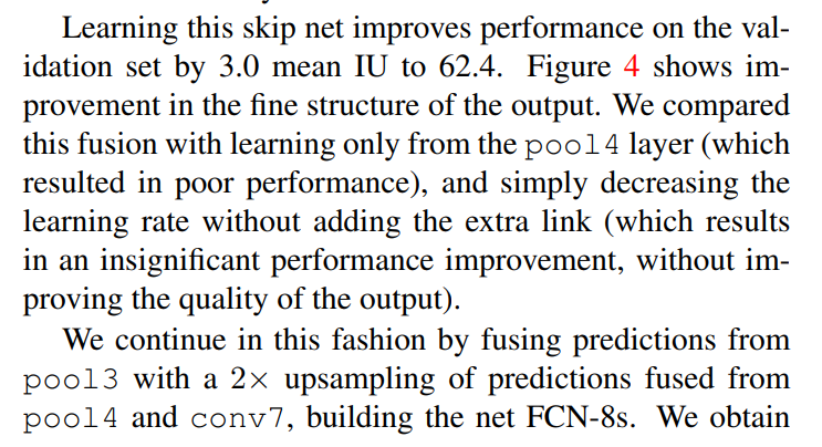
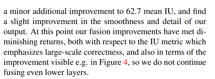
Now that the authors have detailed the “how” of their FCN-16s and FCN-8s architectures, they present the results of these experiments.

The Payoff of FCN-16s

Learning this skip net improves performance on the validation set by 3.0 mean IU to 62.4. Figure 4 shows improvement in the fine structure of the output.

This is a significant result.

• FCN-32s (baseline): 59.4 mIoU (this is the score with extra training data mentioned earlier, making it a stronger baseline to compare against).
• FCN-16s: 62.4 mIoU.

Adding just one skip connection from pool4 provides a solid +3.0 mIoU boost. This is a big jump at the state-of-the-art level. The authors also note that the improvement isn’t just in the numbers; the visual quality (“fine structure”) of the output is noticeably better, which we can see in Figure 4.

To prove that the skip connection itself is what matters, they run two sanity-check experiments:

1. Training only from pool4: This gave “poor performance.” This makes sense. pool4 has good spatial detail but lacks the deep semantic context of the later layers. It knows where edges are, but not what they belong to.
2. Just fine-tuning FCN-32s longer: They tried continuing to train the baseline model with the lower learning rate but without the skip connection. This resulted in “insignificant” improvement.

These checks confirm that the performance gain comes specifically from the fusion of deep and shallow features.

Extending to FCN-8s

Next, they apply the same logic one more time to build the FCN-8s model.

We continue in this fashion by fusing predictions from pool3 with a 2× upsampling of predictions fused from pool4 and conv7, building the net FCN-8s. We obtain a minor additional improvement to 62.7 mean IU, and find a slight improvement in the smoothness and detail of our output.

This is another key result.

• FCN-16s: 62.4 mIoU.
• FCN-8s: 62.7 mIoU.

Adding a second skip connection from pool3 gives another small boost of +0.3 mIoU. The visual quality also gets a little better.

The Law of Diminishing Returns

This result leads them to their final architectural conclusion.

At this point our fusion improvements have met diminishing returns, both with respect to the IU metric which emphasizes large-scale correctness, and also in terms of the improvement visible e.g. in Figure 4, so we do not continue fusing even lower layers.

This is a very important and practical observation.

• The first skip connection (FCN-16s) gave a +3.0 mIoU improvement.
• The second skip connection (FCN-8s) gave a +0.3 mIoU improvement.

The benefit is clearly shrinking. While they could continue this process, adding skip connections from pool2 (FCN-4s) and pool1 (FCN-2s), the engineering complexity would increase for what would likely be a very tiny gain in performance.

The mIoU metric itself also plays a role. It cares more about getting the overall shape and location of the object correct (“large-scale correctness”) than it does about pixel-perfect boundaries. Therefore, the huge gains come from the first skip connection that cleans up the coarse blobs, while further refinements yield smaller and smaller gains on this particular metric.

Based on this, they decide to stop at FCN-8s, which represents the best balance of performance and complexity.

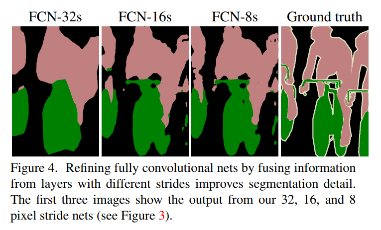
This figure is the perfect illustration of the “what vs. where” tradeoff and how the skip architecture helps to resolve it. It shows the output of the three main architectures—FCN-32s, FCN-16s, and FCN-8s—compared to the ground truth label. The image appears to show a person (pink) on a bicycle (green).

Let’s analyze the progression from left to right.

1. FCN-32s: The Coarse Baseline

• Observation: The output is extremely “blobby” and coarse. The general shapes of the person and the bicycle are there, but the boundaries are smeared and undefined. The thin structures of the bicycle frame and handlebars are completely lost, merged into a single green mass. The person’s arm blends into their torso.
• Interpretation: This is the direct result of making a prediction from the stride-32 feature map. The model has excellent semantic knowledge—it knows that a person and a bicycle are in these general regions—but it has almost zero fine-grained spatial knowledge. The 32x upsampling step cannot possibly recover details that were lost in the deep layers of the network.

2. FCN-16s: The First Leap in Detail

• Observation: There is a dramatic improvement in the level of detail. The boundary between the person and the bicycle is much sharper. We can start to see the shape of the person’s arm and the negative space between their body and the bike. The overall shapes are much less amorphous and closer to the ground truth.
• Interpretation: This is the effect of fusing the stride-16 pool4 features. The pool4 layer still has enough spatial resolution to “remember” where some of these key boundaries are. The network learns to use this information to correct the coarse blobs from the deeper layers. This is the “+3.0 mIoU” jump we saw in the text, and visually, it’s a huge step forward.

3. FCN-8s: Fine-Tuning the Details

• Observation: The improvement from FCN-16s to FCN-8s is more subtle, but it’s definitely there. The edges become even smoother and more accurate. Look at the person’s shoulder, the top of the bicycle’s handlebars, and the space under the person’s arm—these areas are all slightly cleaner and more defined than in the FCN-16s output.
• Interpretation: This shows the effect of the second skip connection from the stride-8 pool3 layer. This layer provides even finer spatial information, allowing the model to make small, final adjustments to the boundaries. This corresponds to the smaller “+0.3 mIoU” gain and confirms the “diminishing returns” the authors mentioned.

4. Ground Truth: The Goal

• Observation: The ground truth shows just how complex the segmentation task is. The bicycle handlebars and frame are extremely thin structures.
• Interpretation: Even the best model, FCN-8s, is not perfect. It still struggles with the thinnest parts of the bicycle and doesn’t capture every nuance of the person’s outline. However, by comparing FCN-32s to FCN-8s, the power of the skip architecture is undeniable. It transforms a coarse, almost useless segmentation into one that is highly detailed and remarkably close to the ground truth.

4.3. Experimental Framework

This section dives into the practical details of how the models were trained. While less glamorous than the architectural innovations, these details are what make the difference between a great idea and a working, state-of-the-art system.

Optimization

This part describes the core training algorithm and its hyperparameters.

• Algorithm: Standard SGD with momentum. This was the workhorse optimizer of the era.
• Batch Size: 20 images per minibatch.
• Learning Rates: They used fixed learning rates, which they found by experimentation (“line search”). Notably, the learning rate for the powerful VGG16 model (10⁻⁴) is much smaller than for AlexNet (10⁻³), which is a common practice when fine-tuning very deep networks.
• Other Hyperparameters: They used standard momentum (0.9) and weight decay. They also used a common trick of doubling the learning rate for bias terms.
• Initialization: They zero-initialize the final classification layer (the 1x1 convolution that produces the class scores). This is a safe and stable choice, and they found that random initialization didn’t help.
• Regularization: They kept Dropout in the network where it existed in the original classifiers (e.g., in the fully connected layers of VGG that were converted to convolutions).

Fine-tuning

This section emphasizes the importance of their training strategy.

• Whole-network fine-tuning: They confirm that they fine-tune all layers of the network, not just the newly added ones. The error signal from the segmentation loss is backpropagated through the entire net.
• Justification: They provide a crucial ablation study: fine-tuning only the final output layer yields just 70% of the performance of full fine-tuning. This proves that the early feature-extraction layers are also adapting to the new task, which is key to achieving top performance.
• No Training from Scratch: They state that training these massive networks from random initialization is not feasible due to the time it would take. Relying on the ImageNet pre-training is essential.
• Training Time: They provide practical numbers: training the baseline FCN-32s takes about three days on a single GPU, and upgrading and fine-tuning it to FCN-16s and then FCN-8s takes about one additional day for each step.

Patch Sampling (vs. Whole Image Training)

Here, they directly address the popular alternative to their whole-image training approach and prove that their method is superior.

• The Theory: Prior work often used random patch sampling, arguing that the higher variance in these batches could speed up convergence.
• The FCN Equivalent: The authors simulate patch sampling in their framework by randomly ignoring the loss from a subset of the output cells (1-p of them). This is a clever form of spatial dropout on the loss itself.
• The Result (Figure 5): The results are crystal clear.
  • Left Plot (vs. Iteration Number): All methods (full image, 50% sampling, 25% sampling) converge at roughly the same rate per iteration. Sampling doesn’t seem to offer a convergence advantage.
  • Right Plot (vs. Wall Clock Time): This is the key. Whole-image training is dramatically faster. Because sampling requires processing more images to form a single effective batch, it takes much longer to reach the same level of performance.
• The Verdict: They conclude that their unsampled, whole-image training is the most effective and efficient strategy.

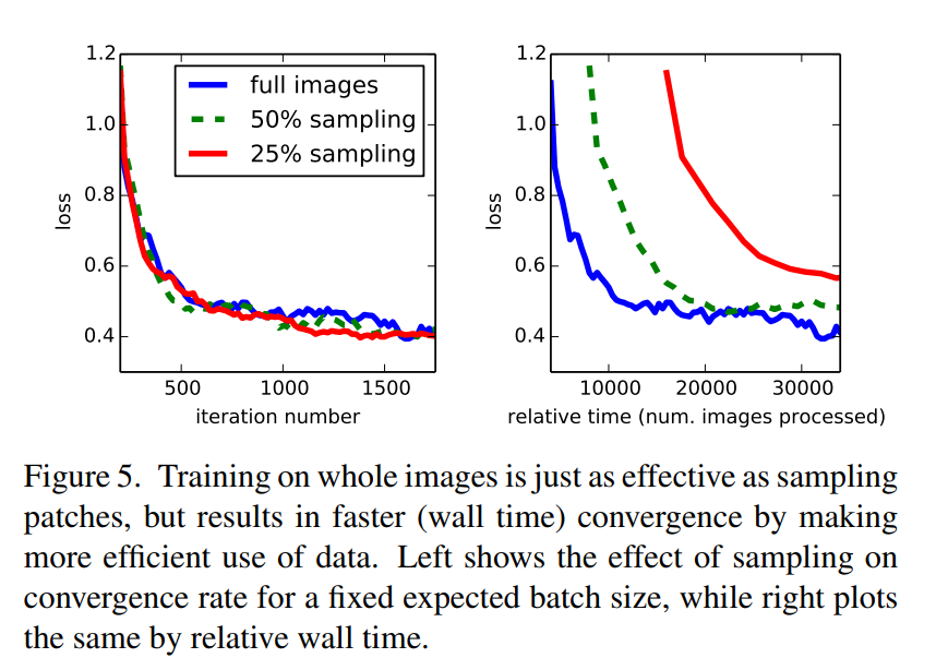
Other Experimental Details

• Class Balancing: They found that although their dataset was mildly imbalanced (mostly background pixels), they did not need to use any special class balancing techniques (like weighting the loss). The standard training worked fine.
• Dense Prediction: They reiterate their upsampling strategy. The final upsampling layer is a fixed bilinear interpolation, but the intermediate upsampling layers (in FCN-16s and FCN-8s) are initialized as bilinear but are then learned. They explicitly state they do not use shift-and-stitch.
• Augmentation: They tried standard data augmentation techniques like random mirroring and jittering (small translations) but found it provided “no noticeable improvement.” This is a somewhat surprising result, but it suggests the pre-trained features are already very robust.
• More Training Data: They mention the two datasets used: the standard PASCAL VOC 2011 training set (1112 images) and a much larger set of 8498 images collected by Hariharan et al., which was used to train the previous state-of-the-art model and is used here for their best results.

5. Results

This section showcases the performance of the authors’ best model, the FCN-8s, on a variety of challenging tasks.

We test our FCN on semantic segmentation and scene parsing, exploring PASCAL VOC, NYUDv2, and SIFT Flow. Although these tasks have historically distinguished between objects and regions, we treat both uniformly as pixel prediction.

This opening statement highlights the generality of their approach. They don’t need different models for “objects” vs. “stuff” (like grass or sky); their FCN treats everything as a pixel classification problem.

Metrics

First, they formally define the evaluation metrics they will use, which are all variations of pixel accuracy and Intersection over Union (IoU). The most important one, as discussed before, is mean IU (mIoU), which is the gold standard.

PASCAL VOC

This is the main event. PASCAL VOC was the most influential object segmentation benchmark at the time.

Table 3 gives the performance of our FCN-8s on the test sets of PASCAL VOC 2011 and 2012, and compares it to the previous state-of-the-art, SDS [16], and the well-known R-CNN [12]. We achieve the best results on mean IU by a relative margin of 20%. Inference time is reduced 114× (convnet only…) or 286× (overall).

Table 3 tells a stunning story of progress.

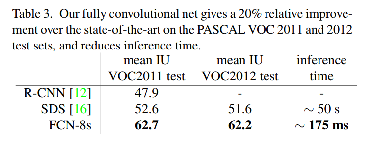
Let’s analyze the breakthrough:

• Massive Accuracy Jump: FCN-8s achieves 62.2 mIoU on the 2012 test set. The previous state-of-the-art, SDS, was at 51.6. This isn’t just a small improvement; it’s a 20% relative leap ((62.2 - 51.6) / 51.6 ≈ 0.20), which is a massive advancement in a mature field.
• Ludicrous Speedup: The FCN model is orders of magnitude faster. SDS took almost a minute per image (50 seconds). The FCN takes 175 milliseconds (less than 1/5th of a second). This is a speedup of roughly 286 times. This speedup is a direct result of the end-to-end, whole-image processing paradigm, which eliminates the need for slow proposal generation and complex post-processing.

NYUDv2

To prove their method isn’t just a one-trick pony, they test it on NYUDv2, an indoor scene segmentation dataset that includes depth information from a Microsoft Kinect sensor (RGB-D).

• The Challenge: How to best incorporate the depth (D) channel along with the color (RGB) channels?
• Experiments: They try several strategies:
  1. RGB only (baseline): Just use the color images.
  2. RGB-D (early fusion): Treat depth as a fourth input channel. This gave little benefit.
  3. HHA: Use a sophisticated pre-processing method from Gupta et al. [14] that converts raw depth into three meaningful channels: Horizontal disparity, Height above ground, and Angle with gravity (HHA).
  4. RGB + HHA (late fusion): Train two separate FCN streams, one for RGB and one for HHA, and add their final prediction scores together. This two-stream “late fusion” model performed the best.
• The Result: Their final model (a 16-stride version, FCN-16s) again achieves state-of-the-art results on this dataset, demonstrating the FCN’s ability to adapt to multi-modal data.

SIFT Flow

Finally, they tackle the SIFT Flow dataset, which has labels for both semantic classes (e.g., “bridge,” “mountain”) and geometric classes (“horizontal,” “vertical,” “sky”).

• The Challenge: Can a single network learn to predict two different types of labels for each pixel simultaneously?
• The Architecture: “Two-headed” FCN. This is a beautiful demonstration of the flexibility of FCNs. They take their FCN-16s and, at the very end, branch it into two separate prediction “heads.”
  • One head is a 1x1 convolution that predicts the 33 semantic classes.
  • The other head is a 1x1 convolution that predicts the 3 geometric classes.
• The Training: The network is trained with a combined loss function that is simply the sum of the semantic loss and the geometric loss. The entire network learns a shared representation in its backbone that is useful for solving both tasks.
• The Result: This multi-task FCN performs as well on both tasks as two models that were trained completely independently. And, because the feature extraction is shared, it’s nearly twice as fast as running two separate models. This is another major win for the FCN paradigm, showing its power in multi-task learning settings.