MobileNetV1 Explained: A Deep Dive into Lightweight Neural Networks

papers

A detailed, page-by-page breakdown of the MobileNetV1 paper, explaining how to build efficient neural networks for mobile and edge devices.

Published

September 2, 2025

Introduction

Ever wonder how your smartphone pulls off those magical AI tricks? Portrait mode that blurs the background perfectly, real-time language translation through your camera, or those fun filters that pop up on your face? These features require a tremendous amount of computation, yet your phone doesn’t get scorching hot or run out of battery in five minutes. How is that possible?

The secret lies in designing neural networks that are not just accurate, but also incredibly efficient. They need to be small enough to fit in your phone’s memory and fast enough to run in real-time. This is a huge challenge, and for a long time, the worlds of top-tier accuracy and on-device performance were far apart.

In 2017, a team at Google published a landmark paper called “MobileNets: Efficient Convolutional Neural Networks for Mobile Vision Applications.” This paper didn’t just introduce a single new model; it presented a brilliant and practical blueprint for building a whole family of lightweight, fast, and powerful models designed specifically for the constraints of mobile and embedded devices.

In this post, we’ll take a guided tour through the MobileNets paper, breaking it down page-by-page. By the end, you’ll understand the simple yet powerful ideas behind its design, why it was so revolutionary, and how its core components have become fundamental building blocks for modern AI.

Let’s start with the abstract.

The Abstract: MobileNets in a Nutshell

A paper’s abstract is its elevator pitch. In just a few sentences, it tells you the problem, the proposed solution, the results, and why it matters. The MobileNets abstract is a perfect example, laying out the entire story concisely.

Here is the abstract from the paper:

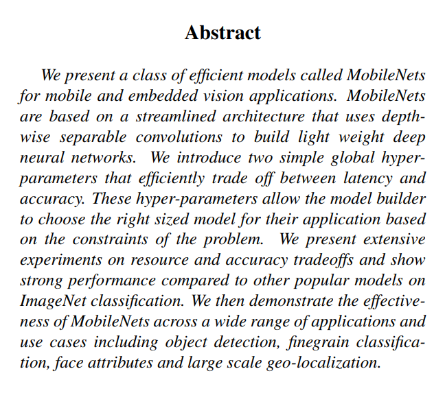
Let’s unpack the key promises made in this short paragraph.

The Goal: To create “efficient models… for mobile and embedded vision applications.” This is the core mission statement.
The Secret Sauce: The key technical idea is an operation called depthwise separable convolutions. This is the magic ingredient that allows them to build networks that are both “light weight” and “deep” (which is crucial for accuracy).
The Killer Feature: They introduce two simple “control knobs” (hyper-parameters) that let any developer easily trade off speed for accuracy. This is incredibly practical. It means you can choose the perfect model for your specific needs—whether you need maximum speed for a live video filter or higher accuracy for an offline photo-sorting app.
The Proof: They don’t just propose an idea; they prove it works. They show strong results on the standard ImageNet benchmark and demonstrate that MobileNets are versatile enough to be used for a wide variety of tasks, from object detection to face analysis.

In essence, the abstract promises a practical, powerful, and proven recipe for building efficient AI. Now, let’s dive into the paper to see how they deliver on these promises.

Why We Need Smarter, Not Just Bigger, AI

The introduction of a paper is crucial. It sets the stage, frames the problem, and tells you why you should care about the solution being proposed. On page 1, the authors of MobileNets walk us through the state of computer vision at the time, painting a clear picture of a field heading in a direction that was unsustainable for mobile applications.

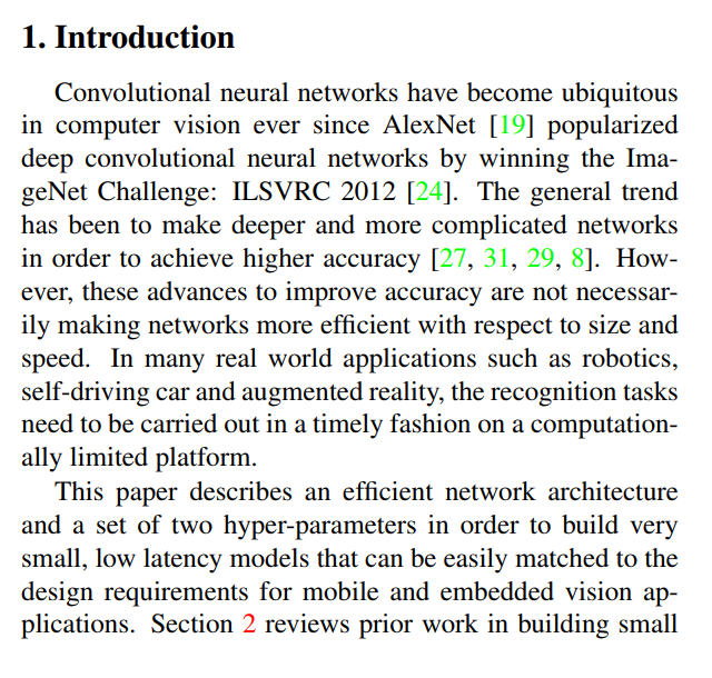
The “Accuracy Arms Race”

The first paragraph takes us back to the years following 2012, a time when deep learning was exploding in popularity thanks to a model called AlexNet. The dominant trend was clear: to get better results, you just had to build bigger and deeper networks. This led to an “arms race” where research labs competed to create massive, complex models that could inch out a new state-of-the-art score on academic benchmarks.

But the authors point out a critical flaw in this approach:

(Page 1, Introduction, Para 1): “The general trend has been to make deeper and more complicated networks in order to achieve higher accuracy… However, these advances to improve accuracy are not necessarily making networks more efficient with respect to size and speed. In many real world applications such as robotics, self-driving car and augmented reality, the recognition tasks need to be carried out in a timely fashion on a computationally limited platform.”

This is the core problem MobileNets was designed to solve. While giant models running on powerful servers in the cloud are great, they are useless for tasks that need to happen right here, right now, on the device in your hand. Your phone, your drone, or the smart camera in your home is a “computationally limited platform.” It doesn’t have endless power or memory. The relentless pursuit of accuracy was leaving these real-world applications behind.

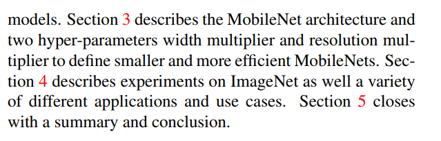
The Blueprint for a Solution

So, how do we break out of this “bigger is better” cycle? The paper’s introduction immediately lays out a clear, two-part plan.

(Page 1, Introduction, Para 2): “This paper describes an efficient network architecture and a set of two hyper-parameters in order to build very small, low latency models that can be easily matched to the design requirements for mobile and embedded vision applications.”

This single sentence is the blueprint for the entire paper. The solution isn’t just one thing; it’s a combination of two powerful ideas:

An Efficient Architecture: They will propose a new way to build the fundamental layers of a neural network, making them inherently faster and smaller from the ground up.
Two Simple Hyper-parameters: They will provide two easy-to-use “control knobs” that allow anyone to customize the architecture. These knobs, which they will later call the width multiplier and the resolution multiplier, give developers the power to fine-tune the trade-off between speed, size, and accuracy for their specific needs.

The introduction does its job perfectly. It establishes a clear tension between the academic trend of building massive networks and the practical need for efficient on-device AI. It then promises a clear, elegant, and customizable solution to resolve that tension.

With the stage set, the paper next takes a look at the “Prior Work”

Standing on the Shoulders of Giants (Prior Work)

Great research rarely happens in a vacuum. Before diving into the technical details of their new architecture, the authors take a moment in Section 2 to survey the landscape of efficient neural network design. This shows they are aware of other approaches and helps us understand exactly where MobileNets fits in and what makes it different.

Two Paths to a Smaller Network

The paper begins by outlining the two main strategies that researchers were using to create smaller, more efficient models.

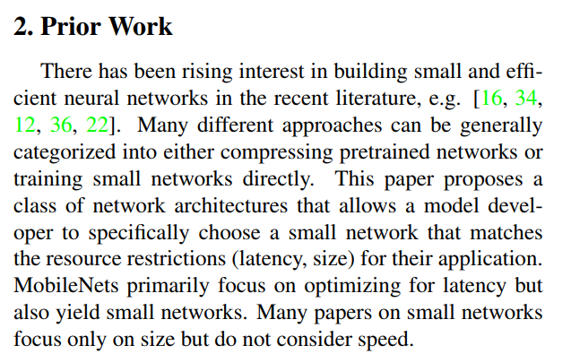
(Page 1, Section 2, Para 1): “Many different approaches can be generally categorized into either compressing pretrained networks or training small networks directly. This paper proposes a class of network architectures that allows a model developer to specifically choose a small network that matches the resource restrictions (latency, size) for their application.”

This is a fantastic, high-level summary. Let’s break down these two paths:

The “Compression” Path: This strategy starts with a big, powerful, pre-trained model (like a VGG or ResNet). Then, it applies a series of clever tricks to shrink it down, like pruning away unimportant connections or using quantization to represent the weights with fewer bits. Think of this as taking a large, high-resolution photo and running it through a compression algorithm to get a smaller JPEG file. You lose some quality, but the file size is much smaller.
The “Efficient Design” Path: This strategy doesn’t start with a big model. Instead, it focuses on designing a network architecture that is small and fast from the very beginning. It’s about building with lighter, more efficient materials from the ground up, rather than trying to slim down a heavyweight construction later.

The authors clearly state that MobileNets belong to the second category. They aren’t a trick to compress big models; they are a fundamentally new recipe for building efficient models from scratch.

A Focus on Speed, Not Just Size

This first paragraph ends with a crucial philosophical point that distinguishes MobileNets from much of the other research at the time.

(Page 1, Section 2, Para 1): “MobileNets primarily focus on optimizing for latency but also yield small networks. Many papers on small networks focus only on size but do not consider speed.”

This is a subtle but incredibly important distinction. Latency is about how fast the model can make a prediction. Size is about how much storage space the model takes up. While the two are often related, they are not the same thing.

A model could be small in file size but use computationally awkward operations that are slow to run on a mobile phone’s processor. The MobileNet team made a conscious decision to prioritize speed (low latency) above all else. Their goal was to design an architecture that was not just theoretically efficient, but one that would be blazingly fast on real hardware. As we’ll see, this focus on practical, real-world speed would guide many of their most important design decisions.

The Building Blocks of Efficiency

The authors now zoom in on the second category of research—designing efficient networks from scratch—and acknowledge the key ideas and contemporary papers that influenced their work. This paragraph is a whirlwind tour of the concepts that were “in the air” at the time.

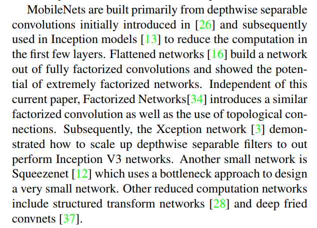
(Page 1, Section 2, Para 2): “MobileNets are built primarily from depthwise separable convolutions initially introduced in [26] and subsequently used in Inception models [13] to reduce the computation in the first few layers…”

This first sentence is the most important. The authors give credit where credit is due, stating that the core component of MobileNets—the depthwise separable convolution—was not their invention. We’ll dive deep into what this operation is in the next section, but for now, the key takeaway is that this efficient building block had been seen before. It was even used in a limited capacity in Google’s own famous Inception models. The big innovation of MobileNets was not in inventing this block, but in recognizing its full potential and building an entire architecture out of it.

The paragraph then lists several other influential approaches to efficient network design:

Factorized Convolutions (Flattened Networks, Factorized Networks): This is the general principle that depthwise separable convolutions are based on. “Factorizing” just means breaking down one big, expensive mathematical operation into several smaller, cheaper ones that approximate the original. These other papers explored different ways of doing this, proving that the core idea was powerful.
The Xception Network: This is a crucial paper that came out shortly before MobileNets. It took the ideas from the Inception family and pushed them to their logical extreme, showing that depthwise separable convolutions could be scaled up to build state-of-the-art models, not just small ones. This provided strong evidence that this was a powerful and general-purpose building block.
SqueezeNet: This was another very famous small network. SqueezeNet’s approach was different; it cleverly used 1x1 convolutions in a “bottleneck” structure to “squeeze” the number of channels down, do some processing, and then expand them back up. This was another very effective way to reduce the number of parameters and computations.

By mentioning all these different papers, the authors show that they are part of a vibrant research community that was actively trying to solve the problem of network efficiency. While SqueezeNet used bottlenecks and Inception used complex multi-path modules, the MobileNet authors placed their bet on a single, elegant idea: what happens if we build an entire deep network using nothing but the simplest and most efficient building block we can find—the depthwise separable convolution?

Tricks of the Trade: Shrinking, Squeezing, and Distilling

To round out their review of prior work, the authors briefly touch on the other major philosophy for creating small models: taking a large, pre-trained network and applying clever techniques to shrink it.

“A different approach for obtaining small networks is shrinking, factorizing or compressing pretrained networks. Compression based on product quantization [36], hashing [2], and pruning, vector quantization and Huffman coding [5] have been proposed in the literature.”

This sounds like a lot of jargon, but the core idea is simple. These are all different methods for “compressing” the information stored in a network’s weights, much like you would compress a large file on your computer.

Pruning: Imagine a dense web of connections in the network. Pruning is like a gardener snipping away the weakest, least important connections, leaving behind a sparse but still effective network.
Quantization: A typical neural network stores its numbers (weights) with high precision (e.g., 32-bit floating point). Quantization is the process of using fewer bits to store these numbers. This can dramatically reduce the model’s file size, often with little loss in accuracy.
Huffman Coding: This is a classic data compression technique (used in things like JPEG and MP3 files) that can be applied to the network’s weights to make the final model file even smaller.

The authors also mention a fascinating and powerful technique that bridges the gap between the “large model” world and the “small model” world.

“Another method for training small networks is distillation [9] which uses a larger network to teach a smaller network. It is complementary to our approach and is covered in some of our use cases in section 4.”

Knowledge Distillation is a beautiful idea. Imagine you have a wise, experienced “teacher” model that is very large and accurate, and a small, nimble “student” model (like a MobileNet).

Instead of training the student on a raw dataset, you have it learn by mimicking the teacher. The teacher provides “soft labels”—not just the final answer, but its confidence and nuances. The student learns to replicate the teacher’s “thought process,” effectively transferring the knowledge from the large model into its own compact form.

The authors astutely point out that this is complementary to their work. MobileNet is the perfect “student” architecture for distillation. They even foreshadow that they will use this exact technique in their experiments later in the paper.

With this survey complete, the stage is now perfectly set. We understand the problem (the need for efficient on-device AI), the two main schools of thought for solving it (compression vs. efficient design), and where MobileNets fits in. Now, it’s time to dive into the technical heart of the paper: the MobileNet architecture itself.

MobileNet Architecture

Now we get to the heart of the paper: the MobileNet architecture itself. In Section 3, the authors introduce the brilliant and efficient building block that makes the entire system work: the depthwise separable convolution.

This sounds complicated, but the core idea is beautifully simple. It’s about taking the standard, workhorse operation of computer vision—the convolution—and breaking it apart into two smaller, much faster steps.

First, the paper gives us a quick roadmap for the section.

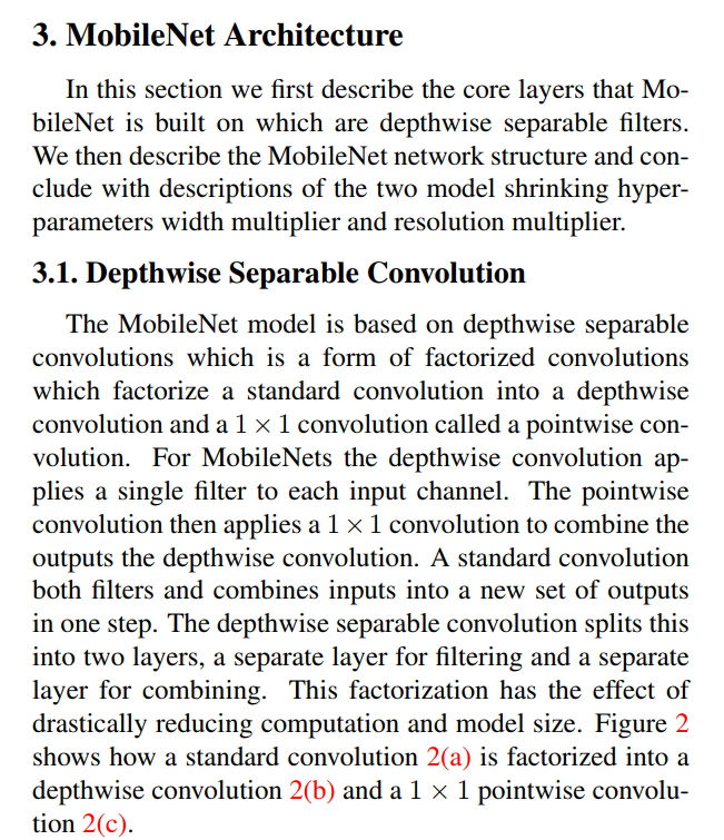
(Page 2, Section 3, Intro): “In this section we first describe the core layers that MobileNet is built on which are depthwise separable filters. We then describe the MobileNet network structure and conclude with descriptions of the two model shrinking hyper-parameters width multiplier and resolution multiplier.”

They’ll start with the fundamental building block, then show how it’s assembled into a full network, and finally explain the “control knobs” used to customize it.

The Two Jobs of a Standard Convolution

Before we can understand the MobileNet way, we need to understand what a standard convolution does. A standard convolution is a powerhouse, but it’s trying to do two very different jobs at the same time:

It filters spatially: It scans over an image to find spatial patterns, like edges, corners, textures, or shapes.
It combines channels: It mixes information from the input channels to create new, meaningful features in the output channels.

The MobileNet paper argues that forcing one single operation to do both of these jobs at once is inefficient. The key insight is to “separate” these responsibilities.

The MobileNet Way: Divide and Conquer

This brings us to the core concept of the paper, explained in the first paragraph of Section 3.1.

(Page 2, Section 3.1, Para 1): “The MobileNet model is based on depthwise separable convolutions which is a form of factorized convolutions which factorize a standard convolution into a depthwise convolution and a 1 × 1 convolution called a pointwise convolution… A standard convolution both filters and combines inputs into a new set of outputs in one step. The depthwise separable convolution splits this into two layers, a separate layer for filtering and a separate layer for combining.”

This is the entire trick in a nutshell. Instead of one big, expensive layer, MobileNet uses two small, cheap layers:

The Depthwise Convolution (The “Filtering” Step): This first layer handles only the spatial filtering. It glides a filter over the input, but it does so for each input channel independently. It doesn’t mix information between channels at all. If the input has 64 channels, this step produces 64 filtered channels, keeping them all separate.
The Pointwise Convolution (The “Combining” Step): This second layer handles the channel mixing. It uses a brilliantly simple and fast 1x1 convolution. This tiny filter looks at a single pixel and intelligently combines the values from all the channels produced by the depthwise step to create a new, rich feature.

This “factorization”—splitting one big job into two specialized smaller jobs—is the key. The paper states the outcome in no uncertain terms:

(Page 2, Section 3.1, Para 1): “This factorization has the effect of drastically reducing computation and model size.”

This is the secret sauce. By separating the concerns of filtering and combining, MobileNets achieve a massive reduction in the number of calculations and parameters needed. As we’ll see in the next section, this isn’t just a small improvement; it makes the operation about 8 to 9 times more efficient than a standard convolution, with almost no loss in accuracy. This is the breakthrough that makes fast, powerful on-device AI possible.

The Math of the Bottleneck: Why Standard Convolutions Are So Expensive

To truly appreciate the elegance of the MobileNet solution, we first need to understand the problem in more detail. Why, exactly, is a standard convolution so computationally expensive? The paper now dives into the math to give us a clear answer.

The authors start by defining the pieces involved in a standard convolution layer.

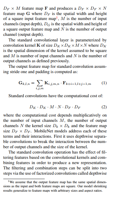
(Page 2, Section 3.1, Para 2-4): A standard convolutional layer takes as input a D_F × D_F × M feature map F and produces a D_G × D_G × N feature map G… The standard convolutional layer is parameterized by convolution kernel K of size D_K × D_K × M × N…

Let’s quickly translate this math-speak:

Input Feature Map (F): This is the input data for the layer. It has a Height (D_F), a Width (D_F), and a number of Channels (M). For the very first layer of a network, this would be your image, and M would be 3 (for Red, Green, and Blue).
Output Feature Map (G): This is what the layer produces. It has a Height and Width and a new number of Channels (N).
Kernel (K): This is the filter that slides over the input. Its size is D_K × D_K. A common size is 3x3.

The Cost Formula That Changes Everything

Now we get to the most important equation in this section, which calculates the total computational cost of a single standard convolution layer.

(Page 2, Equation 2): Computational Cost = D_K · D_K · M · N · D_F · D_F

This formula looks intimidating, but it’s the key to everything. It tells us that the total number of multiplication operations is the product of:

D_K · D_K: The size of our filter (e.g., 3x3 = 9).
M: The number of channels in our input.
N: The number of channels we want in our output.
D_F · D_F: The size of our input feature map.

The crucial insight is that all these terms are multiplied together. Let’s look at the part of the formula that creates the bottleneck:

... M · N ...

The cost is directly proportional to the number of input channels (M) multiplied by the number of output channels (N). In a deep neural network, these numbers can be very large (e.g., 256, 512, or even 1024). When you multiply two large numbers together, the result is huge. This M x N term is what causes the computational cost to explode.

As the paper states, this is exactly what MobileNet is designed to fix:

(Page 2, Section 3.1, Para 5): “MobileNet models address each of these terms and their interactions. First it uses depthwise separable convolutions to break the interaction between the number of output channels and the size of the kernel.”

The phrase “break the interaction” is key. The genius of the depthwise separable convolution is that it restructures the operation so that M and N are no longer multiplied together in the most expensive part of the calculation.

Now that we’ve seen the “before” picture—the math of the expensive standard convolution—we’re perfectly set up to see the “after” picture: the math that makes MobileNets so incredibly efficient.

The Math of Efficiency, Step 1: The Depthwise Filter

Now that we understand why standard convolutions are so costly, we can finally appreciate the genius of the MobileNet approach. The authors now present the math for their two-step “divide and conquer” strategy, and the savings become immediately obvious.

Let’s look at the first step, the depthwise convolution, which handles the spatial filtering.

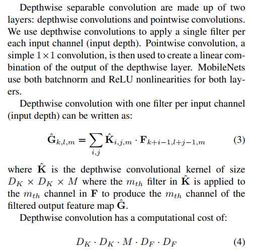
(Page 3, Section 3.1, Para 1): “Depthwise separable convolution are made up of two layers: depthwise convolutions and pointwise convolutions. We use depthwise convolutions to apply a single filter per each input channel (input depth)…”

This confirms what we discussed earlier. The first step’s job is to filter each channel on its own, without mixing them. If you have an input with 64 channels, this step will use 64 separate filters, one for each channel.

The New, Cheaper Cost Formula

The paper then presents the computational cost for just this depthwise filtering step.

(Page 3, Equation 4): Depthwise Cost = D_K · D_K · M · D_F · D_F

Let’s compare this to the original, expensive cost formula from the standard convolution:

Original Cost: D_K · D_K · M · N · D_F · D_F
New Depthwise Cost: D_K · D_K · M · D_F · D_F

The difference is immediately clear. The N term is gone!

Why? Because in this step, we are no longer trying to create N new output channels. We are simply filtering the existing M input channels, so we only need M filters.

The impact of removing N (the number of output channels, which can be a large number like 512) is massive. This single change makes the depthwise filtering step N times cheaper than a full standard convolution.

This is a huge first step, but it’s not the whole story. As the paper points out, this layer is efficient but incomplete. It only filters the input channels; it doesn’t combine them to create new, more complex features. That’s the job of the second step: the pointwise convolution. But already, we can see how “breaking the interaction” has led to a dramatic reduction in computational cost.

The Math of Efficiency, Step 2: The Pointwise Combination and the Final Payoff

We’ve seen that the first step, the depthwise convolution, is incredibly efficient. But as the paper notes, it’s an incomplete solution.

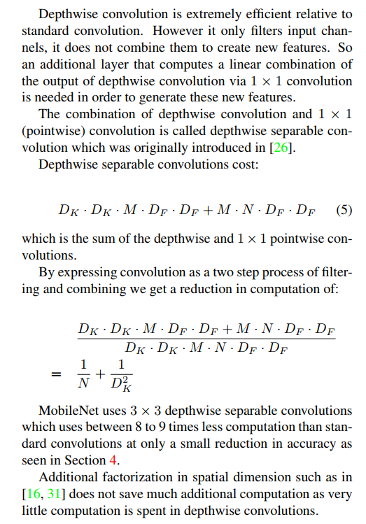
(Page 3, Section 3.1, Para 2): “However it only filters input channels, it does not combine them to create new features. So an additional layer that computes a linear combination of the output of depthwise convolution via a 1 × 1 convolution is needed in order to generate these new features.”

This is where the second part of the block comes in: the pointwise convolution. Its job is to take the independently filtered channels from the first step and intelligently mix them together to create a new set of meaningful features. This layer uses a brilliantly simple 1x1 convolution to accomplish this.

The Total Cost of Efficiency

The paper now presents the total computational cost of the complete two-step depthwise separable convolution. It’s simply the cost of the depthwise step plus the cost of the pointwise step.

(Page 3, Equation 5): Total Cost = (D_K · D_K · M · D_F · D_F) + (M · N · D_F · D_F)

Part 1 (Depthwise Cost): The first term is the cost of filtering, which we already saw is very cheap.
Part 2 (Pointwise Cost): The second term is the cost of combining. It’s the cost of a standard convolution, but with the filter size D_K set to 1, making it highly efficient.

Tip

A Quick Note: Where does the pointwise cost (M·N·D_F·D_F) come from?

A pointwise convolution is just a special case of a standard convolution where the kernel size is 1x1.

Remember the original cost formula for a standard convolution?

Standard Cost = D_K · D_K · M · N · D_F · D_F

If we set our kernel size D_K = 1 for the pointwise step, the formula becomes:

Pointwise Cost = 1 · 1 · M · N · D_F · D_F

…which simplifies to exactly M · N · D_F · D_F. It’s the same math, just applied to a tiny 1x1 filter, which is what makes it so fast.

Now for the moment of truth. How does this new, two-part cost compare to the original, expensive cost of a standard convolution? The paper shows the ratio:

(Page 3, The Ratio Equation): (New Cost) / (Old Cost) = 1/N + 1/D_K²

This simple, elegant formula is the punchline of the entire architectural design. It tells you exactly how much more efficient the MobileNet block is. Let’s plug in some typical numbers:

MobileNets almost always use 3x3 filters, so D_K = 3, which means D_K² = 9.
The number of output channels N is usually a large number, like 128, 256, or 512. This makes the 1/N term very, very small (close to zero).

This means the cost ratio is approximately 1/9.

The authors state this incredible result in plain English:

(Page 3, Section 3.1, Final Para): “MobileNet uses 3 × 3 depthwise separable convolutions which uses between 8 to 9 times less computation than standard convolutions at only a small reduction in accuracy…”

This is the breakthrough. By cleverly splitting one operation into two, MobileNets achieve a nearly 9x reduction in computational cost. And as their experiments will show, they do this while sacrificing almost no accuracy. This is the fundamental trade-off that makes MobileNets so powerful and is the key reason they can run so effectively on devices with limited computational power.

Assembling the Architecture: A Blueprint for Efficiency

Having established the power of their core building block—the depthwise separable convolution—the authors now zoom out in Section 3.2 to show us how these blocks are stacked together to create the full, 28-layer MobileNet.

The design philosophy is one of simplicity and uniformity, using modern best practices to create a clean and effective structure.

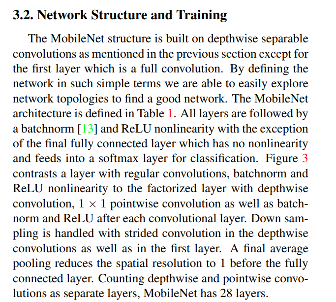
(Page 3, Section 3.2, Para 1): “The MobileNet structure is built on depthwise separable convolutions as mentioned in the previous section except for the first layer which is a full convolution… All layers are followed by a batchnorm and ReLU nonlinearity…”

This paragraph gives us a high-level overview of the network’s construction, which we can break down into a few key principles:

Uniformity is Key: The network is simply a deep stack of the depthwise separable blocks we just learned about. This clean, repeating pattern makes the architecture easy to understand, scale, and implement. The only exception is the very first layer, which uses a standard convolution. This is a common trick to quickly process the input image and expand its channel depth, creating a rich set of features for the more efficient blocks to work with.
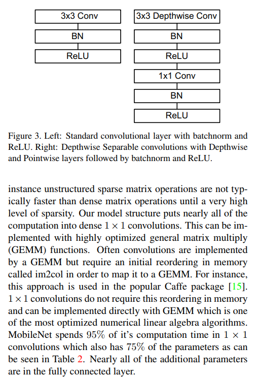
Modern Ingredients: Every convolutional layer (both depthwise and pointwise) is followed by two standard and essential components of modern deep learning:
- BatchNorm (Batch Normalization): Think of this as a regulator for the data flowing through the network. It keeps the numbers in a healthy range, which dramatically stabilizes and speeds up the training process.
- ReLU (Rectified Linear Unit): This is the network’s non-linearity. It’s a very simple operation (it just clips all negative values to zero) that allows the network to learn complex, non-linear patterns.
Efficient Downsampling: As an image progresses through a network, its spatial dimensions (height and width) are gradually reduced. Older networks often used separate “pooling” layers for this. MobileNet uses a more modern and efficient technique: strided convolutions. By setting the stride to 2 in some of the depthwise layers, the network downsamples the feature map and learns new features at the same time, killing two birds with one stone.
A Smart Finish: At the very end of the network, instead of flattening the final high-dimensional feature map (which would create a huge number of parameters), MobileNet uses global average pooling. This simple operation averages each channel down to a single value, creating a compact feature vector that is then fed to the final classifier. This is a highly efficient and effective way to finish the network.

In summary, the MobileNet architecture is an elegant and straightforward stack of its core efficient blocks, seasoned with all the right modern ingredients (BatchNorm, ReLU, strided convolutions, and global average pooling) to make it a robust and high-performing network.

From Theory to Reality: Designing for Real Hardware

Having a low theoretical operation count is great, but it’s only half the story. To build a truly fast network, you have to consider the nuts and bolts of how the calculations are actually performed on a physical CPU or GPU. The MobileNet authors display their deep engineering expertise here, explaining how their design is not just mathematically efficient, but also perfectly tailored for modern hardware.

As the authors wisely state:

(Page 3, Section 3.2, Para 2): “It is not enough to simply define networks in terms of a small number of Mult-Adds. It is also important to make sure these operations can be efficiently implementable.”

This is a golden rule of performance engineering. Some operations are just easier for computer chips to execute quickly. The genius of MobileNet is that its design concentrates the vast majority of its work into the single most hardware-friendly operation available: the 1x1 convolution.

The Superpower of the 1x1 Convolution

Why is a 1x1 convolution so special? Because it is mathematically equivalent to a GEMM (General Matrix Multiply) operation.

While “GEMM” might sound like a fancy acronym, it’s just a highly optimized, standardized way of performing matrix multiplication. Matrix multiplication is the single most studied and optimized operation in all of scientific computing. Hardware vendors and software engineers have spent decades creating libraries (like Intel’s MKL and NVIDIA’s cuBLAS) that make this operation run at blistering speeds.

(Page 4, Section 3.2, Para 1): “Our model structure puts nearly all of the computation into dense 1 × 1 convolutions. This can be implemented with highly optimized general matrix multiply (GEMM) functions.”

This is the key. While a standard 3x3 convolution can be turned into a GEMM operation, it requires a slow and memory-hungry preparation step called im2col. A 1x1 convolution, on the other hand, does not need this step. It can be mapped directly to a GEMM call, making it incredibly fast and memory-efficient.

The authors then deliver the knockout punch with some stunning statistics from their architecture (which they detail in Table 2).

(Page 4, Section 3.2, Para 1): “MobileNet spends 95% of it’s computation time in 1 × 1 convolutions which also has 75% of the parameters…”

This is a masterful piece of engineering. They designed an architecture where:

The vast majority of the work (95% of the computation!) is concentrated in the most efficient, hardware-friendly operation possible (the 1x1 convolution).
The less-optimized part (the 3x3 depthwise convolution) is so cheap that it barely registers in the total runtime.

This is the difference between an architecture that is merely theoretically efficient and one that is practically fast. By understanding the underlying hardware, the MobileNet team designed a network that wasn’t just smart on paper—it was built for speed in the real world.

The Art of Training: Less is More for Small Models

Having a great architecture is one thing, but you still need to train it effectively. In this section, the authors share some fascinating insights they discovered about the best way to train their new, lightweight MobileNets. The key takeaway? When it comes to training small models, sometimes less is more.

A Different Set of Rules for Small Models

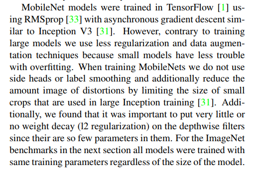
The team started with a standard, powerful training setup used for giant models like Inception V3. But they quickly realized that this aggressive approach wasn’t right for their smaller MobileNets.

(Page 4, Section 3.2, Para 2): “However, contrary to training large models we use less regularization and data augmentation techniques because small models have less trouble with overfitting.”

This is the central insight. Overfitting is a major concern for large models. They have so much capacity that they can easily “memorize” the training data instead of learning general patterns. To combat this, researchers use heavy regularization and data augmentation—techniques that make the training task harder to prevent the model from memorizing.

But small models are different. A MobileNet simply doesn’t have enough parameters to memorize the entire dataset. It is naturally more resistant to overfitting. Therefore, the heavy-handed techniques used for large models are not only unnecessary, they can actually be harmful. It’s like trying to train for a marathon by running with a 100-pound backpack—it’s overkill and can prevent you from learning to run properly.

The authors found that MobileNets train best with a “gentler” touch:

Less Augmentation: They reduced the amount of image distortion used during training, such as limiting the size of small, random crops.
No Advanced Regularization: They removed complex regularization tricks like “label smoothing” and “side heads,” which are often needed to tame massive models.
Careful Weight Decay: They discovered that applying a standard penalty on large weights (called weight decay or L2 regularization) to the tiny depthwise filters was a bad idea. These filters have very few parameters, and penalizing them too much prevented them from learning useful features.

This is a brilliant lesson in the art of machine learning. The best training recipe is not one-size-fits-all. A small, efficient model like MobileNet benefits from a more direct and less aggressive training strategy, allowing it to learn the essential patterns in the data without being held back by unnecessarily harsh regularization.

The Blueprint and the Receipt: A Look at the Numbers

Theory is great, but seeing the actual architecture laid out provides a new level of clarity. On page 4, the paper presents two crucial tables. Table 1 is the blueprint for the standard MobileNet, showing its layer-by-layer construction. Table 2 is the receipt, detailing the computational cost and parameter distribution, and it perfectly illustrates why the MobileNet design is so brilliant.

Table 1: The MobileNet Blueprint

This table is the complete, layer-by-layer specification for the baseline MobileNet. While it looks dense, it reveals a clean, logical, and repeating pattern.

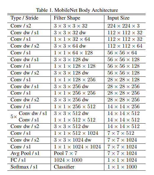
By reading down the columns, we can trace the journey of an image through the network:

The Start: The network begins with a standard 3x3 convolution (Conv / s2), which takes the 224x224x3 input image and immediately halves its size to 112x112 while increasing the channels to 32.
The Core Block: The rest of the network is a repeating sequence of our new favorite block: a Conv dw (depthwise) followed by a Conv (which is always a 1x1 pointwise convolution). This pattern is the heart of MobileNet.
Shrinking and Growing: As we go deeper, the spatial dimensions get progressively smaller (224 -> 112 -> 56 -> 28 -> 14 -> 7), while the number of channels (the depth) gets progressively larger (32 -> 64 -> 128 -> … -> 1024). This is a classic and effective design for CNNs.
The Finish: The network ends with a Avg Pool (Global Average Pooling) and a final FC (Fully Connected) layer for classification.

This blueprint shows a clean, deep, and highly structured architecture built almost entirely from a single, repeating, efficient block.

Tip

You might have noticed the s1 and s2 in the “Type / Stride” column. This is a shorthand that tells us something very important about how the layer operates: its stride.

s1 means a stride of 1. The filter moves one pixel at a time. It slides from one position to the very next, examining every single location meticulously.
- Effect on Image Size: The output feature map will have the same height and width as the input (assuming a bit of padding is added around the edges). It preserves the spatial dimensions.
s2 means a stride of 2. The filter takes a bigger step, moving two pixels at a time. It effectively skips every other pixel.
- Effect on Image Size: The output feature map will be roughly half the height and half the width of the input. This is a very efficient way to shrink or downsample the data.

The strategic use of s1 and s2 is a key part of the architecture’s intelligence:

Layers with s1 are used when the network wants to learn more complex features at the current scale. For example, in the middle of the network (the 5x block), all the convolutions use s1 because the goal is to get much smarter about the 14x14 feature maps without shrinking them.
Layers with s2 are used at transition points, when the network is ready to summarize the information it has learned and move to a coarser level of detail. This also has a massive benefit for efficiency: by halving the height and width, you quarter the number of pixels, which drastically reduces the computational cost for all the layers that come after it.

Here’s a quick summary:

Notation	Meaning	Effect on Image Size	Purpose in MobileNet
s1	Stride 1	Preserves Size	Learn richer features at the same scale.
s2	Stride 2	Halves Size	Downsample and reduce computational cost.

This clever mix of s1 and s2 layers allows MobileNet to build up a deep understanding of an image while progressively and efficiently reducing its size.

Table 2: The Receipt - Where the Money is Spent

This second table is the punchline for the entire architectural design. It answers the question: “In this new design, where do the computations and parameters actually live?” The results are stunning.

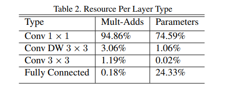
Let’s break down this “receipt”:

Conv 1 × 1 (Pointwise): The Workhorse
- This layer accounts for a staggering 94.86% of the computation and 74.59% of the parameters. This is the masterful engineering trick we discussed earlier. MobileNet is designed to spend almost all of its time and resources on the 1x1 convolution, which is the single operation that can be executed most efficiently on modern hardware (via GEMM).
Conv DW 3 × 3 (Depthwise): The “Almost Free” Filter
- In contrast, the spatial filtering part of the block is incredibly cheap. It accounts for a tiny 3.06% of the computation and a negligible 1.06% of the parameters. This is the entire justification for separating the convolution: the expensive part is isolated into this almost-free operation.
Fully Connected: Heavy but Not Slow
- The final classifier layer holds a significant chunk of the parameters (24.33%), but because it only runs once at the very end on a small vector, it consumes a trivial 0.18% of the computation.

These two tables, the blueprint and the receipt, provide the ultimate proof of concept. The MobileNet architecture isn’t just a clever idea; it’s a meticulously engineered system that successfully shifts the computational burden onto the most efficient operations possible, resulting in a network that is both powerful and incredibly fast.

The Control Knobs, Part 1: The Width Multiplier for Thinner Models

We’ve seen the brilliant architecture and the smart training strategy. But what truly makes MobileNets a game-changer for developers is its customizability. The paper now introduces the first of two simple yet powerful “control knobs” that allow you to create the perfect-sized model for any application.

This first knob is called the width multiplier, and its job is to make the network “thinner.”

One Knob to Rule Them All

The baseline MobileNet is already small and fast, but what if you need something even smaller and even faster for a particularly demanding task, like real-time augmented reality on a low-end phone?

(Page 4, Section 3.3, Para 1): “In order to construct these smaller and less computationally expensive models we introduce a very simple parameter α called width multiplier. The role of the width multiplier α is to thin a network uniformly at each layer.”

The idea is incredibly simple and elegant. The width multiplier, represented by the Greek letter alpha (α), is a single number (between 0 and 1) that uniformly reduces the number of channels in every single layer of the network.

For example, if you choose α = 0.5:

A layer that originally had 64 channels will now have 0.5 * 64 = 32 channels.
A layer that had 128 channels will now have 0.5 * 128 = 64 channels.

You simply decide on a value for α, and the entire network is scaled down proportionally. This is a much more principled way to shrink a network than just randomly removing layers.

The Power of Quadratic Scaling

Here’s where things get really interesting. When you make the network half as “wide,” you might expect it to become twice as efficient. But the effect is much more dramatic. The paper reveals a crucial mathematical insight:

(Page 4, Section 3.3, Para 2): “Width multiplier has the effect of reducing computational cost and the number of parameters quadratically by roughly α².”

This is the punchline. The cost doesn’t scale linearly; it scales quadratically (by α²).

Let’s see what that means in practice:

If you set α = 0.75, the cost is reduced by 0.75² ≈ 0.56. The model becomes almost twice as fast.
If you set α = 0.5, the cost is reduced by 0.5² = 0.25. The model becomes four times as fast and has four times fewer parameters.
If you set α = 0.25, the cost is reduced by 0.25² ≈ 0.06. The model becomes over 16 times as fast.

This quadratic scaling gives developers an incredibly powerful tool. With one simple number, you can generate a whole spectrum of models, from the full-sized, most accurate version (α = 1.0) down to tiny, lightning-fast versions, all while knowing that you’re shrinking the network in a smart, uniform way.

It’s important to note, as the paper points out, that you use the width multiplier to define a new, smaller architecture that must then be trained from scratch. But now, let’s look at the second control knob, which works in a completely different but equally powerful way.

The Control Knobs, Part 2: The Resolution Multiplier for Faster Processing

The width multiplier (α) gives us a powerful way to make a network thinner. But the MobileNet authors provide a second, complementary control knob that is even more intuitive: the resolution multiplier.

The idea is incredibly simple: if you want the network to run faster, just feed it a smaller image!

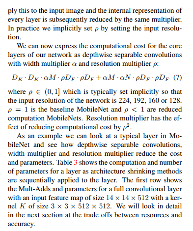
(Page 4, Section 3.4, Para 1): “The second hyper-parameter to reduce the computational cost of a neural network is a resolution multiplier ρ. We apply this to the input image and the internal representation of every layer is subsequently reduced by the same multiplier.”

The resolution multiplier, represented by the Greek letter rho (ρ), isn’t a number you set directly. Instead, you “implicitly” set it by choosing the input resolution for your images.

The baseline resolution is 224x224 (ρ = 1.0).
If you choose to use 192x192 images, you’ve implicitly set ρ ≈ 0.857.
If you choose to use 160x160 images, you’ve implicitly set ρ ≈ 0.714.

This size reduction at the input then propagates through the entire network, making every single feature map smaller and faster to process.

Another Quadratic Win

Just like the width multiplier, the resolution multiplier has a powerful quadratic effect on the computational cost.

(Page 5, Section 3.4, Para 2): “Resolution multiplier has the effect of reducing computational cost by ρ².”

This is because the computation is proportional to the number of pixels in the feature maps, which is height × width. When you reduce both the height and width by a factor of ρ, the total number of pixels is reduced by ρ².

Example: If you switch from 224x224 images to 160x160 (ρ ≈ 0.714), you reduce the computational cost by a factor of ρ² ≈ 0.51. You’ve cut the work the network has to do in half just by giving it a smaller picture to look at.

The Grand Finale: Putting It All Together

The paper provides a brilliant summary in Table 3, showing the compounding effect of all these efficiency innovations on a single, typical layer from the middle of the network. This table is the ultimate “before and after” picture.

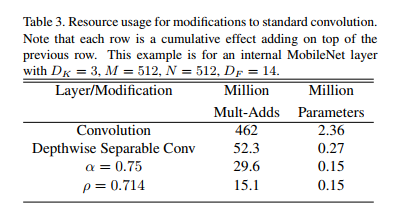
Let’s walk through it step-by-step, seeing how each modification slashes the cost:

Baseline (Standard Convolution): We start with an old-school, standard 3x3 convolution. For this one layer, it costs a massive 462 Million Mult-Adds and requires 2.36 Million parameters.
Add Depthwise Separable Conv: We swap the standard convolution for the efficient MobileNet block. The cost plummets to 52.3M Mult-Adds and 0.27M parameters. That’s a nearly 9x reduction in computation, right off the bat!
Add Width Multiplier (α = 0.75): Now, we make the layer “thinner.” The cost drops again to 29.6M Mult-Adds, a further reduction of almost half, just as the α² rule predicted.
Add Resolution Multiplier (ρ = 0.714): Finally, we process a smaller feature map through this thinner layer. The cost is halved one more time, down to a mere 15.1M Mult-Adds.

The final result is staggering. A layer that would have cost 462 Million operations in a traditional CNN now costs just 15 Million in a scaled-down MobileNet. That’s a 30-fold reduction in computation.

This powerful combination—an efficient core block and two simple, intuitive control knobs—is what gives developers the unprecedented ability to design a network that perfectly fits the performance constraints of any device. With the theory now fully explained, the paper turns to the experiments to prove that these models aren’t just efficient, but also highly accurate.

The Experiments, Part 1: Putting the Theory to the Test

The theory behind MobileNets is elegant, the math is compelling, but the ultimate question is always: does it actually work? And how well does it work compared to other approaches? In Section 4, the paper shifts from design to rigorous experimentation, providing the hard data to justify its core ideas.

The first set of experiments in Section 4.1 is designed to answer two fundamental questions:

Is the depthwise separable convolution really a good trade-off?
Is making a network “thinner” truly better than making it “shallower”?

Justifying the Secret Sauce: Is the Trade-Off Worth It?

First, the authors need to prove that their core building block is a smart choice. Is the massive gain in efficiency worth the potential drop in accuracy? To find out, they compare two models: a “Conv MobileNet” built with expensive standard convolutions, and the real MobileNet built with their efficient blocks. The results in Table 4 are a knockout.

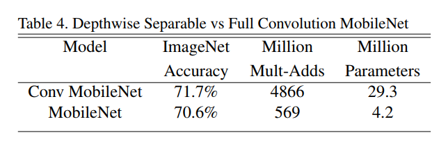
(Page 5, Section 4.1, Para 1-2): “First we show results for MobileNet with depthwise separable convolutions compared to a model built with full convolutions. In Table 4 we see that using depthwise separable convolutions compared to full convolutions only reduces accuracy by 1% on ImageNet was saving tremendously on mult-adds and parameters.”

Let’s break down that trade-off:

The Cost: They sacrificed a mere 1.1% in ImageNet accuracy (71.7% -> 70.6%).
The Reward: In return, they got a network that was ~8.5 times faster (fewer Mult-Adds) and ~7 times smaller (fewer Parameters).

This is a phenomenal result. It’s like being offered a car that’s 99% as fast as a supercar but gets 8 times the gas mileage and costs 7 times less. It’s an overwhelmingly positive trade-off and the ultimate validation of the paper’s core premise.

A Smarter Way to Shrink: Thinner vs. Shallower

Next, the authors justify their choice of the “width multiplier.” If you have a fixed computational budget, what’s a better way to make a model smaller?

Make it thinner by reducing the number of channels in every layer?
Or make it shallower by removing entire layers from the network?

To answer this, they create two models with a nearly identical computational budget: a “thinner” MobileNet (using α = 0.75) and a “shallower” MobileNet (with 5 layers removed from the middle).

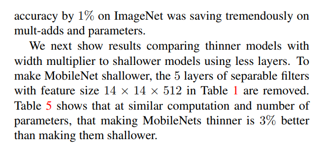
(Page 5, Section 4.1, Para 3): “Table 5 shows that at similar computation and number of parameters, that making MobileNets thinner is 3% better than making them shallower.”

The results from Table 5 were decisive. For the same computational cost, the thinner model was 3.1% more accurate than the shallower one.

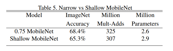
This is a crucial design lesson. It suggests that maintaining the network’s depth is vital for its performance. It’s better to have many “thin” layers than a few “fat” ones. This experiment provides the perfect justification for using the width multiplier as the primary, principled way to scale down the MobileNet architecture.

These two initial experiments are foundational. They prove that MobileNet’s core building block is a massive win and that the proposed method for scaling it (making it thinner) is the right approach.

The Experiments, Part 2: A Universe of Efficient Models

Having justified their core design choices, the authors now unleash the full power of their two “control knobs”—the width and resolution multipliers. This section demonstrates how these simple hyper-parameters create a rich ecosystem of 16 different models, allowing developers to find the perfect balance of speed, size, and accuracy for any conceivable task.

Mapping the Trade-Offs: The Power of Predictable Scaling

First, the paper presents the results of applying each knob independently.

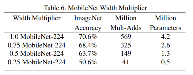
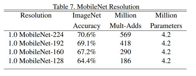
Table 6 (The Width Multiplier α): This table shows what happens as you make the network progressively “thinner” by decreasing α from 1.0 down to 0.25. The key finding is that the accuracy “drops off smoothly.” This is fantastic news. It means the trade-off is graceful and predictable. There are no sudden, catastrophic drops in performance, allowing a developer to confidently tune the knob to meet their latency budget.
Table 7 (The Resolution Multiplier ρ): This table shows the results of shrinking the input image size from 224x224 down to 128x128. The story is the same: accuracy “drops off smoothly across resolution.” Again, this provides a predictable and reliable way to gain speed.

But the real magic happens when you combine them. Figure 4 is the ultimate summary of the MobileNet family’s performance.

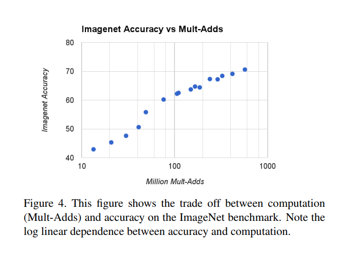
This single graph plots all 16 models, showing the relationship between their computational cost (Mult-Adds) and their accuracy. The key takeaway is the shape of the curve: on this plot with a logarithmic x-axis, the points form an almost perfectly straight line.

This “log-linear” relationship is a developer’s dream. It means that for every multiplicative decrease in speed (e.g., making the model 10x faster), you get a predictable, additive decrease in accuracy (e.g., losing 15% accuracy). This turns the art of choosing a model into a science. You can look at this chart and say, “My phone has a budget of 100 Million Mult-Adds; I can expect to get about 63% accuracy.”

Figure 5 tells the other half of the story, plotting accuracy against model size (number of parameters).

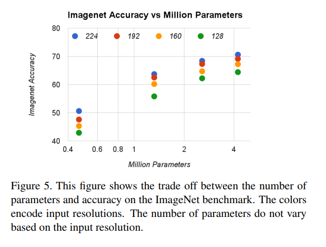
This chart shows that model size is determined only by the width multiplier α, creating distinct vertical clusters. Within each size budget, you can then use the resolution multiplier to further trade latency for accuracy. Together, these two figures provide a complete map for navigating the MobileNet universe.

The Main Event: MobileNet vs. The World

So, how do these new, efficient models stack up against the famous architectures of the day? The paper provides a head-to-head comparison in Table 8 and Table 9.

Table 8 compares the full-size baseline MobileNet to the heavyweights:

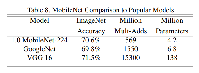
vs. VGG16: MobileNet achieves nearly the same accuracy (70.6% vs. 71.5%) while being 32 times smaller and 27 times faster. This is a revolutionary leap in efficiency.
vs. GoogLeNet: MobileNet is more accurate, smaller, and over 2.5 times faster. It’s a clean sweep.

But what about the smaller MobileNet variants? Table 9 compares a shrunk-down MobileNet (α=0.5, 160x160 resolution) to other models famous for their small size:

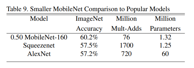
vs. AlexNet: The small MobileNet is 3% more accurate while being 45 times smaller and 9.4 times faster.
vs. SqueezeNet: SqueezeNet was a celebrated small model. Yet, the small MobileNet is nearly 3% more accurate at the same size, while being a staggering 22 times faster in terms of computation.

The conclusion from these tables is undeniable. The MobileNet family doesn’t just create a single good model; it establishes a new state-of-the-art across the entire spectrum of performance. Whether you need a full-size competitor to VGG or a tiny model to rival SqueezeNet, the MobileNet architecture provides a superior solution. It proved that efficiency and high performance were not mutually exclusive.

Beyond Classification: A Versatile Tool for the Real World

Having firmly established MobileNet’s dominance on the standard ImageNet benchmark, the paper spends the remainder of the experiments section (Sections 4.3 through 4.7) demonstrating its incredible versatility. The goal is to prove that MobileNet isn’t just a one-trick pony for classification; it’s a powerful and efficient “backbone” that can be adapted to a wide variety of real-world computer vision tasks.

The authors put MobileNet to the test on a diverse set of challenges, and it excels in every single one. Here’s a quick summary of the highlights:

Fine-Grained Recognition (Stanford Dogs dataset): MobileNet proves it can handle the subtle and difficult task of distinguishing between 120 different breeds of dogs, achieving near state-of-the-art results with a fraction of the computational cost.
Large-Scale Geolocalization (PlaNet): When used as a drop-in replacement for the massive Inception V3 model in the PlaNet system (which determines where a photo was taken), MobileNet delivers nearly the same performance while being 4 times smaller and 10 times faster.
Face Attributes: Using a powerful technique called “knowledge distillation,” the authors show they can train a tiny MobileNet to mimic a huge, complex in-house face attribute model. The result is a model that performs just as well as the original but is up to 100 times more efficient.
Object Detection (COCO dataset): When integrated into modern object detection systems like SSD and Faster R-CNN, MobileNet achieves comparable results to much larger backbones like VGG and Inception V2, but with a dramatic reduction in complexity and speed.
Face Embeddings (FaceNet): Finally, they show that a MobileNet-based model can be trained to generate high-quality facial recognition embeddings, rivaling the famous FaceNet model but in a package small enough for mobile deployment.

The message from these experiments is loud and clear: MobileNet is a universally effective feature extractor. Its efficiency does not come at the cost of its ability to learn powerful and generalizable representations of the visual world.

Conclusion: The Legacy of MobileNet

The MobileNet paper is more than just a description of a clever architecture. It’s a masterclass in principled, practical, and impactful research. By starting from a simple yet powerful insight—that the two core jobs of a convolution can be separated—the authors created not just a single model, but an entire philosophy for designing efficient neural networks.

Let’s recap the journey:

The Core Idea: They replaced the expensive, monolithic standard convolution with a lightweight, two-part alternative called the depthwise separable convolution, achieving a nearly 9x gain in efficiency with minimal loss in accuracy.
Smart Design: They built a clean, deep architecture that was not only theoretically efficient but also meticulously engineered to run at maximum speed on real hardware by concentrating its workload on highly optimized 1x1 convolutions.
Unprecedented Flexibility: They introduced two simple but powerful “control knobs”—the width and resolution multipliers—that allow any developer to easily generate a whole family of models, finding the perfect trade-off between speed, size, and accuracy for their specific needs.
Proven Performance: Through extensive experiments, they proved that MobileNets outperform their larger, more cumbersome predecessors and are a versatile tool that excels at a wide range of computer vision tasks, from object detection to facial recognition.