Detect Vanishing Gradients in Deep Neural Networks by Plotting Gradient Distributions

In this notebook, we will explore how vanishing gradients can affect the training of a deep neural network. We will visualize the gradient flow from the deeper to starting layers during the backpropagation for two popular activation functions, Sigmoid and ReLU.

Credits

This notebook takes inspiration and ideas from the following sources.

• A great post from MATLAB company MathWorks with the same title: Detect Vanishing Gradients in Deep Neural Networks by Plotting Gradient Distributions. That post is written for the MATLAB audience, and I have tried translating its ideas for Python and PyTorch community.
• The outstanding book “Deep Learning with PyTorch Step-by-Step” by “Daniel Voigt Godoy”. You can get the book from its website: pytorchstepbystep. In addition, the GitHub repository for this book has valuable notebooks and can be used independently: github.com/dvgodoy/PyTorchStepByStep. Parts of the code you see in this notebook are taken from chapter 3 notebook of the same book.
• University of Amsterdam (UvA) Deep Learning Course series. uvadlc.github.io. Their lecture on “activation functions and gradients” discusses the same topic. Here is the link: tutorial3/Activation_Functions.html. The course is outstanding, and lectures and notebooks are also openly shared. From the course site “This course is taught in the MSc program in Artificial Intelligence of the University of Amsterdam. In this course we study the theory of deep learning, namely of modern, multi-layered neural networks trained on big data.”

Environment

This notebook is prepared with Google Colab.

• GitHub: 2022-10-23-pytorch-vanishing-gradients-deep-neural-networks.ipynb
• Open In Colab:

Code

from platform import python_version
import numpy, matplotlib, pandas, torch, seaborn

print("python==" + python_version())
print("numpy==" + numpy.__version__)
print("torch==" + torch.__version__)
print("matplotlib==" + matplotlib.__version__)
print("seaborn==" + seaborn.__version__)

python==3.7.15
numpy==1.21.6
torch==1.12.1+cu113
matplotlib==3.2.2
seaborn==0.11.2

Introduction

MathWorks post explains vanishing gradients problem in deep neural networks really well, and I am sharing a passage from it.

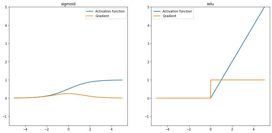
A common problem in deep network training is vanishing gradients. Deep learning training algorithms aim to minimize the loss by adjusting the network’s learnable parameters (i.e., weights) during training. Gradient-based training algorithms determine the level of adjustment using the gradients of the loss function with respect to the current learnable parameters. The gradient computation uses the propagated gradients from the previous layers for earlier layers (i.e., from the output layer to the input layer). Therefore, when a network contains activation functions that always produce gradient values less than 1 (e.g., Sigmoid), the value of the gradients can become increasingly small as the updating algorithm moves toward the initial layers. As a result, early layers in the network can receive a vanishingly small gradient, and therefore, the network is unable to learn. However, if the gradient of the activation function is always greater than or equal to 1 (e.g., ReLU), the gradients can flow through the network, reducing the chance of vanishing gradients.

Let’s understand it better by visualizing the gradients produced by Sigmoid and ReLU.

Compare activation functions

In this section we will compare the properties of two popular activation functions: Sigmoid and ReLU.

Sigmoid

Sigmoid function is normally used to refer specifically to the logistic function, also called the logistic sigmoid function. It is defined as

\[ Sigmoid(x) = \frac{\mathrm{1} }{\mathrm{1} + e^{-x} } \]

ReLU

ReLU function is defined as

\[ Relu(x) = max(0,x) \]

Visualising activation functions and their gradients

Let’s plot both these functions’ outputs and visualize their gradients. In the next cell, I have created two PyTorch classes that define Sigmoid and ReLU activations.

Code

import torch.nn as nn

# A class representing Sigmoid activation function
class SigmoidAct(nn.Module):
    def __init__(self):
        super().__init__()
        pass

    def forward(self, x):
        return 1 / (1 + torch.exp(-x))

# A class representing ReLU activation function
class ReluAct(nn.Module):
    def __init__(self):
        super().__init__()
        pass

    def forward(self, x):
        return x * (x > 0).float()

# initialize sigmoid activation function
sigmoid_fn = SigmoidAct()
# initialize relu activation function
relu_fn = ReluAct()

I have defined a helper function to calculate the gradients for these activation functions.

Code

import matplotlib.pyplot as plt

# A helper function to computes the gradients of an activation function at specified positions.
def get_grads(act_fn, x):
    x = x.clone().requires_grad_()  # Mark the input as tensor for which we want to store gradients
    out = act_fn(x)
    out.sum().backward()  # Summing results in an equal gradient flow to each element in x
    return x.grad  # Accessing the gradients of x by "x.grad"

# A helper function to plot the activation function and its gradient
def vis_act_fn(act_fn, fn_name, ax, x):
    # Run activation function
    y = act_fn(x)
    y_grads = get_grads(act_fn, x)
    # Push x, y and gradients back to cpu for plotting
    x, y, y_grads = x.cpu().numpy(), y.cpu().numpy(), y_grads.cpu().numpy()
    # Plotting
    ax.plot(x, y, linewidth=2, label="Activation function")
    ax.plot(x, y_grads, linewidth=2, label="Gradient")
    ax.set_title(fn_name)
    ax.legend()
    ax.set_ylim(-1.5, x.max())

let’s plot the gradients.

Code

import torch

x = torch.linspace(-5, 5, 1000)

fig, ax = plt.subplots(1, 2, figsize=(15, 7))
vis_act_fn(sigmoid_fn, 'sigmoid', ax[0], x)
vis_act_fn(relu_fn, 'relu', ax[1], x)
fig.subplots_adjust(hspace=0.3)
plt.show()

We can take the following explanations from the above plots.

• The sigmoid output is bounded, as it remains between 0 and 1. The gradients are the highest when the input is close to zero and diminishes as the input value moves away from it. Notice that the sigmoid gradient curve is less than 1 for the entire range; therefore, a network containing sigmoid activation functions can suffer from a vanishing gradients problem.
• The output value for ReLU is not bounded. It keeps on increasing on the positive side. And for positive output values, the gradients do not diminish but remain constant at 1. As the gradient is not decreasing, it reduces the chances of the vanishing gradients problem. However, the gradient is zero for negative values, and this state is sometimes referred to as dead ReLU. It means that if ReLU ends up in this situation, it is improbable that it will recover from it.
  • Why will it not recover? Because the gradient from the activation function is zero for negative inputs, it will also not update the weights during the backward pass, thus leaving the weights in that perpetual state.

In the coming sections, we will build networks and try to visualize how gradients flow between different layers and the effect of activation functions on them.

Section I

I have split the notebook into two sections. In this first section, we will create two multi-layer models: one with sigmoids and the other with ReLU. We will train them on MNIST data and plot their losses. Then in the next section, we will plot their gradients to see how activation functions can affect the behavior of a model.

Download MNIST dataset

MNIST dataset can be downloaded easily from PyTorch built-in datasets provided under torchvision.datasets. In this section, we will download it, split it into train and test datasets, and then convert them into PyTorch tensors.

• Read more about the PyTorch MNIST dataset here
• torchvision.transforms.Compose is like a container to hold a list of transformations you intend to apply. Read more about it here
• torchvision.transforms.ToTensor converts a PIL Image or numpy.ndarray to tensor. It converts a PIL Image or numpy.ndarray (H x W x C) in the range [0, 255] to a torch.FloatTensor of shape (C x H x W) in the range [0.0, 1.0]. Here C=Channel, H=Height, W=Width. Read more about this transformation here

#collapse-output
import torchvision
import numpy as np

train_dataset = torchvision.datasets.MNIST('classifier_data', train=True, download=True)
test_dataset  = torchvision.datasets.MNIST('classifier_data', train=False, download=True)

transform = torchvision.transforms.Compose([
    torchvision.transforms.ToTensor()
])

train_dataset.transform=transform
test_dataset.transform=transform

print(f"Total training images: {len(train_dataset)}")
print(f"Shape of an image: {np.shape(train_dataset.data[7])}")

Downloading http://yann.lecun.com/exdb/mnist/train-images-idx3-ubyte.gz
Downloading http://yann.lecun.com/exdb/mnist/train-images-idx3-ubyte.gz to classifier_data/MNIST/raw/train-images-idx3-ubyte.gz

Extracting classifier_data/MNIST/raw/train-images-idx3-ubyte.gz to classifier_data/MNIST/raw

Downloading http://yann.lecun.com/exdb/mnist/train-labels-idx1-ubyte.gz
Downloading http://yann.lecun.com/exdb/mnist/train-labels-idx1-ubyte.gz to classifier_data/MNIST/raw/train-labels-idx1-ubyte.gz

Extracting classifier_data/MNIST/raw/train-labels-idx1-ubyte.gz to classifier_data/MNIST/raw

Downloading http://yann.lecun.com/exdb/mnist/t10k-images-idx3-ubyte.gz
Downloading http://yann.lecun.com/exdb/mnist/t10k-images-idx3-ubyte.gz to classifier_data/MNIST/raw/t10k-images-idx3-ubyte.gz

Extracting classifier_data/MNIST/raw/t10k-images-idx3-ubyte.gz to classifier_data/MNIST/raw

Downloading http://yann.lecun.com/exdb/mnist/t10k-labels-idx1-ubyte.gz
Downloading http://yann.lecun.com/exdb/mnist/t10k-labels-idx1-ubyte.gz to classifier_data/MNIST/raw/t10k-labels-idx1-ubyte.gz

Extracting classifier_data/MNIST/raw/t10k-labels-idx1-ubyte.gz to classifier_data/MNIST/raw

Total training images: 60000
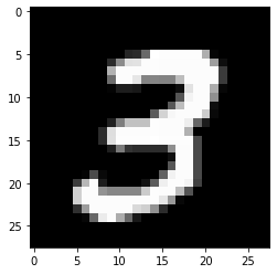
Shape of an image: torch.Size([28, 28])

From the above cell output, there are 60,000 training images. The shape of each image is 28 x 28, which means it is a 2D matrix.

##
# plot a single image
import matplotlib.pyplot as plt

plt.imshow(train_dataset.data[7], cmap='gray')

<matplotlib.image.AxesImage at 0x7fb77b73b590>

Load generated data into PyTorch Dataset and DataLoader class

Now let’s load our data into Dataset and DataLoader classes. PyTorch Dataset is a helper class that converts data and labels into a list of tuples. DataLoader is another helper class to create batches from Dataset tuples. batch_size means the number of tuples we want in a single batch. We have used 128 here, so each fetch from DataLoader will give us a list of 128 tuples.

import torch
from torch.utils.data import Dataset, DataLoader, random_split

train_size=len(train_dataset)

# Randomly split the data into non-overlapping train and validation set
# train size = 70% and validation size = 30%
train_data, val_data = random_split(train_dataset, [int(train_size*0.7), int(train_size - train_size*0.7)])

batch_size=128

# Load data into DataLoader class
train_loader = torch.utils.data.DataLoader(train_dataset, batch_size=batch_size)
valid_loader = torch.utils.data.DataLoader(val_data, batch_size=batch_size)

print(f"Batches in Train Loader: {len(train_loader)}")
print(f"Batches in Valid Loader: {len(valid_loader)}")

print(f"Examples in Train Loader: {len(train_loader.sampler)}")
print(f"Examples in Valid Loader: {len(valid_loader.sampler)}")

Batches in Train Loader: 469
Batches in Valid Loader: 141
Examples in Train Loader: 60000
Examples in Valid Loader: 18000

Define a class to implement training, validation, and mini-batch processing pipeline

In this section we will implement a class that encapsulates all the usual steps required in training a PyTorch model. This way we can focus more on the model architecture and performance, and less concerned about the boilerplate training loop. Important parts of this class are

• __init__: Class constructor to define the main actors in a training cycle including model, optimizer, loss function, training and validation DataLoaders
• _make_train_step_fn: Training pipeline is usually called “training step” which includes the following steps
  1. Compute our model’s predicted output - the forward pass
  2. Compute the loss
  3. Compute gradients i.e., find the direction and scale to update the weights to reduce the loss
  4. Update weight parameters using gradients and the learning rate
• _make_val_step_fn: Validation pipeline is usually called the “validation step” which includes the following steps
  1. Compute our model’s predicted output - the forward pass
  2. Compute the loss
  3. Note that during validation, we are only concerned about the loss, i.e., how well our model performs on the validation dataset. Therefore, we don’t use it to calculate the gradients.
• _mini_batch: It defines the steps to process a single minibatch in a helper function. For a mini-batch processing, we want to
  1. Get the next batch of data and labels (x, y) from the DataLoader iterator
  2. Perform a step on the batch. A step can be either training or validation
  3. Compute the average batch loss
• train: Execute training and validation steps for given number of epoch
• predict: Make a prediction from model on provided data

Code

class DeepLearningPipeline(object):
    def __init__(self, model, loss_fn, optimizer):
        # Here we define the attributes of our class
        
        # We start by storing the arguments as attributes 
        # to use them later
        self.model = model
        self.loss_fn = loss_fn
        self.optimizer = optimizer
        self.device = 'cuda' if torch.cuda.is_available() else 'cpu'
        # Let's send the model to the specified device right away
        self.model.to(self.device)

        # These attributes are defined here, but since they are
        # not informed at the moment of creation, we keep them None
        self.train_loader = None
        self.val_loader = None
        self.writer = None
        
        # These attributes are going to be computed internally
        self.losses = []
        self.val_losses = []
        self.total_epochs = 0
        self.grad = []

        # Creates the train_step function for our model, 
        # loss function and optimizer
        # Note: there are NO ARGS there! It makes use of the class
        # attributes directly
        self.train_step_fn = self._make_train_step_fn()
        # Creates the val_step function for our model and loss
        self.val_step_fn = self._make_val_step_fn()

    def set_loaders(self, train_loader, val_loader=None):
        # This method allows the user to define which train_loader (and val_loader, optionally) to use
        # Both loaders are then assigned to attributes of the class
        # So they can be referred to later
        self.train_loader = train_loader
        self.val_loader = val_loader

    def _make_train_step_fn(self):
        # This method does not need ARGS... it can refer to
        # the attributes: self.model, self.loss_fn and self.optimizer
        
        # Builds function that performs a step in the train loop
        def perform_train_step_fn(x, y):
            # Sets model to TRAIN mode
            self.model.train()

            # Step 1 - Computes our model's predicted output - forward pass
            yhat = self.model(x)
            # Step 2 - Computes the loss
            loss = self.loss_fn(yhat, y)
            # Step 3 - Computes gradients for both "a" and "b" parameters
            loss.backward()
            # Step 4 - Updates parameters using gradients and the learning rate
            self.optimizer.step()
            self.optimizer.zero_grad()

            # Returns the loss
            return loss.item()

        # Returns the function that will be called inside the train loop
        return perform_train_step_fn
    
    def _make_val_step_fn(self):
        # Builds function that performs a step in the validation loop
        def perform_val_step_fn(x, y):
            # Sets model to EVAL mode
            self.model.eval()

            # Step 1 - Computes our model's predicted output - forward pass
            yhat = self.model(x)
            # Step 2 - Computes the loss
            loss = self.loss_fn(yhat, y)
            # There is no need to compute Steps 3 and 4, 
            # since we don't update parameters during evaluation
            return loss.item()

        return perform_val_step_fn
            
    def _mini_batch(self, validation=False):
        # The mini-batch can be used with both loaders
        # The argument `validation`defines which loader and 
        # corresponding step function is going to be used
        if validation:
            data_loader = self.val_loader
            step_fn = self.val_step_fn
        else:
            data_loader = self.train_loader
            step_fn = self.train_step_fn

        if data_loader is None:
            return None
            
        # Once the data loader and step function, this is the 
        # same mini-batch loop we had before
        mini_batch_losses = []
        for x_batch, y_batch in data_loader:
            x_batch = x_batch.to(self.device)
            y_batch = y_batch.to(self.device)

            mini_batch_loss = step_fn(x_batch, y_batch)
            mini_batch_losses.append(mini_batch_loss)

        loss = np.mean(mini_batch_losses)
        return loss

    def set_seed(self, seed=42):
        torch.backends.cudnn.deterministic = True
        torch.backends.cudnn.benchmark = False    
        torch.manual_seed(seed)
        np.random.seed(seed)
    
    def train(self, n_epochs, seed=42):
        # To ensure reproducibility of the training process
        self.set_seed(seed)

        for epoch in range(n_epochs):
            # Keeps track of the numbers of epochs
            # by updating the corresponding attribute
            self.total_epochs += 1

            # inner loop
            # Performs training using mini-batches
            loss = self._mini_batch(validation=False)
            self.losses.append(loss)

            ##########################
            # get grad at the end of each epoch
            imgs, labels = next(iter(self.train_loader))
            imgs, labels = imgs.to(device), labels.to(device)

            # Pass one batch through the network, and calculate the gradients for the weights
            self.model.zero_grad()
            preds = self.model(imgs)
            loss = torch.nn.functional.cross_entropy(preds, labels)
            loss.backward()
            # We limit our visualization to the weight parameters and exclude the bias to reduce the number of plots
            grads = {
                name: params.grad.data.view(-1).cpu().clone().numpy()
                for name, params in self.model.named_parameters()
                if "weight" in name
            }
            self.model.zero_grad()
            self.grad.append(grads)
            ##########################

            # VALIDATION
            # no gradients in validation!
            with torch.no_grad():
                # Performs evaluation using mini-batches
                val_loss = self._mini_batch(validation=True)
                self.val_losses.append(val_loss)

            # If a SummaryWriter has been set...
            if self.writer:
                scalars = {'training': loss}
                if val_loss is not None:
                    scalars.update({'validation': val_loss})
                # Records both losses for each epoch under the main tag "loss"
                self.writer.add_scalars(main_tag='loss',
                                        tag_scalar_dict=scalars,
                                        global_step=epoch)
            
            print(f"epoch: {epoch:3}, train loss: {loss:.5f}, valid loss: {val_loss:.5f}")

        if self.writer:
            # Closes the writer
            self.writer.close()

    def predict(self, x):
        # Set is to evaluation mode for predictions
        self.model.eval() 
        # Takes aNumpy input and make it a float tensor
        x_tensor = torch.as_tensor(x).float()
        # Send input to device and uses model for prediction
        y_hat_tensor = self.model(x_tensor.to(self.device))
        # Set it back to train mode
        self.model.train()
        # Detaches it, brings it to CPU and back to Numpy
        return y_hat_tensor.detach().cpu().numpy()

    def plot_losses(self):
        fig = plt.figure(figsize=(10, 4))
        plt.plot(self.losses, label='Training Loss', c='b')
        plt.plot(self.val_losses, label='Validation Loss', c='r')
        plt.yscale('log')
        plt.xlabel('Epochs')
        plt.ylabel('Loss')
        plt.legend()
        plt.tight_layout()
        return fig

Create a model with sigmoid activations

Let’s define a fully connected 4 layers model with only sigmoid activations.

import torch.nn as nn

SigmoidNet = nn.Sequential()
SigmoidNet.add_module("F", nn.Flatten())
SigmoidNet.add_module("L1", nn.Linear(28*28, 10, bias=False))
SigmoidNet.add_module("S1", nn.Sigmoid())
SigmoidNet.add_module("L2", nn.Linear(10, 10, bias=False))
SigmoidNet.add_module("S2", nn.Sigmoid())
SigmoidNet.add_module("L3", nn.Linear(10, 10, bias=False))
SigmoidNet.add_module("S3", nn.Sigmoid())
SigmoidNet.add_module("L4", nn.Linear(10, 10, bias=False))

Print model’s summary.

torch.manual_seed(42)
device = torch.device("cuda" if torch.cuda.is_available() else "cpu")

#collapse-output
from torchsummary import summary

model_sigmoid = SigmoidNet
model_sigmoid = model_sigmoid.to(device)

summary(model_sigmoid, (1, 28*28))

----------------------------------------------------------------
        Layer (type)               Output Shape         Param #
================================================================
           Flatten-1                  [-1, 784]               0
            Linear-2                   [-1, 10]           7,840
           Sigmoid-3                   [-1, 10]               0
            Linear-4                   [-1, 10]             100
           Sigmoid-5                   [-1, 10]               0
            Linear-6                   [-1, 10]             100
           Sigmoid-7                   [-1, 10]               0
            Linear-8                   [-1, 10]             100
================================================================
Total params: 8,140
Trainable params: 8,140
Non-trainable params: 0
----------------------------------------------------------------
Input size (MB): 0.00
Forward/backward pass size (MB): 0.01
Params size (MB): 0.03
Estimated Total Size (MB): 0.04
----------------------------------------------------------------

Create an optimizer and a loss function.

import torch.optim as optim

# learning rate
lr = 0.001

# Defines a SGD optimizer to update the parameters
optimizer_sigmoid = optim.SGD(model_sigmoid.parameters(), lr=lr)

# Defines a BCE loss function
loss_fn = nn.CrossEntropyLoss()

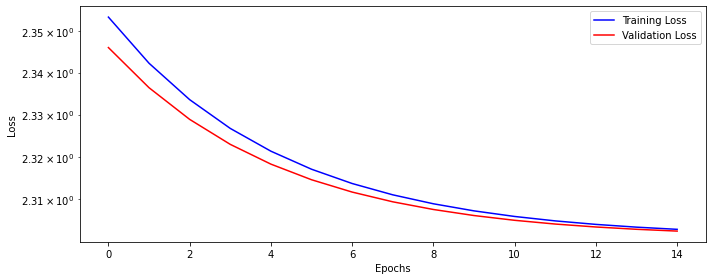
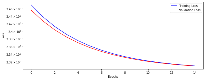
Train our model for 15 epochs.

#collapse-output
n_epochs = 15

dlp_sigmoid = DeepLearningPipeline(model_sigmoid, loss_fn, optimizer_sigmoid)
dlp_sigmoid.set_loaders(train_loader, valid_loader)
dlp_sigmoid.train(n_epochs)

epoch:   0, train loss: 2.38803, valid loss: 2.34602
epoch:   1, train loss: 2.37269, valid loss: 2.33644
epoch:   2, train loss: 2.36004, valid loss: 2.32891
epoch:   3, train loss: 2.34957, valid loss: 2.32299
epoch:   4, train loss: 2.34085, valid loss: 2.31831
epoch:   5, train loss: 2.33357, valid loss: 2.31463
epoch:   6, train loss: 2.32746, valid loss: 2.31172
epoch:   7, train loss: 2.32232, valid loss: 2.30943
epoch:   8, train loss: 2.31798, valid loss: 2.30762
epoch:   9, train loss: 2.31431, valid loss: 2.30620
epoch:  10, train loss: 2.31119, valid loss: 2.30508
epoch:  11, train loss: 2.30853, valid loss: 2.30420
epoch:  12, train loss: 2.30627, valid loss: 2.30351
epoch:  13, train loss: 2.30433, valid loss: 2.30297
epoch:  14, train loss: 2.30266, valid loss: 2.30254

Let’s see how our training and validation loss looks like.

fig = dlp_sigmoid.plot_losses()

Create a model with ReLU activations

This time let’s define the same model with ReLU activation functions.

ReluNet = nn.Sequential()
ReluNet.add_module("F", nn.Flatten())
ReluNet.add_module("L1", nn.Linear(28*28, 10, bias=False))
ReluNet.add_module("S1", nn.ReLU())
ReluNet.add_module("L2", nn.Linear(10, 10, bias=False))
ReluNet.add_module("S2", nn.ReLU())
ReluNet.add_module("L3", nn.Linear(10, 10, bias=False))
ReluNet.add_module("S3", nn.ReLU())
ReluNet.add_module("L4", nn.Linear(10, 10, bias=False))

Print the model’s summary.

#collapse-output
model_relu = ReluNet
model_relu = model_relu.to(device)

summary(model_relu, (1, 28*28))

----------------------------------------------------------------
        Layer (type)               Output Shape         Param #
================================================================
           Flatten-1                  [-1, 784]               0
            Linear-2                   [-1, 10]           7,840
              ReLU-3                   [-1, 10]               0
            Linear-4                   [-1, 10]             100
              ReLU-5                   [-1, 10]               0
            Linear-6                   [-1, 10]             100
              ReLU-7                   [-1, 10]               0
            Linear-8                   [-1, 10]             100
================================================================
Total params: 8,140
Trainable params: 8,140
Non-trainable params: 0
----------------------------------------------------------------
Input size (MB): 0.00
Forward/backward pass size (MB): 0.01
Params size (MB): 0.03
Estimated Total Size (MB): 0.04
----------------------------------------------------------------

Create an optimizer and a loss function.

lr = 0.001

# Defines a SGD optimizer to update the parameters
optimizer_relu = optim.SGD(model_relu.parameters(), lr=lr)

# Defines a BCE loss function
loss_fn = nn.CrossEntropyLoss()

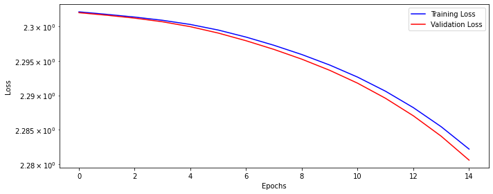
Train the model for 15 epochs.

#collapse-output
n_epochs = 15

dlp_relu = DeepLearningPipeline(model_relu, loss_fn, optimizer_relu)
dlp_relu.set_loaders(train_loader, valid_loader)
dlp_relu.train(n_epochs)

epoch:   0, train loss: 2.30268, valid loss: 2.30202
epoch:   1, train loss: 2.30229, valid loss: 2.30165
epoch:   2, train loss: 2.30193, valid loss: 2.30122
epoch:   3, train loss: 2.30147, valid loss: 2.30069
epoch:   4, train loss: 2.30086, valid loss: 2.29998
epoch:   5, train loss: 2.30012, valid loss: 2.29905
epoch:   6, train loss: 2.29906, valid loss: 2.29793
epoch:   7, train loss: 2.29775, valid loss: 2.29667
epoch:   8, train loss: 2.29621, valid loss: 2.29525
epoch:   9, train loss: 2.29440, valid loss: 2.29363
epoch:  10, train loss: 2.29227, valid loss: 2.29176
epoch:  11, train loss: 2.28972, valid loss: 2.28957
epoch:  12, train loss: 2.28673, valid loss: 2.28703
epoch:  13, train loss: 2.28323, valid loss: 2.28408
epoch:  14, train loss: 2.27912, valid loss: 2.28062

Now plot the model losses.

fig = dlp_relu.plot_losses()

Section II

This section will be more interesting than the last one. Here we will visualize and plot gradients from the trained models and understand their meanings.

Gradients for a model with Sigmoid activations

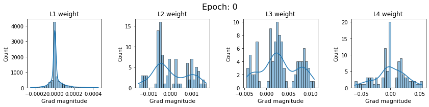
Let’s create a helper function that will plot the gradients for all the weights from each epoch. Note that our models have 4 layers, with L1 being the input layer and L4 being the output layer. Information flows from L1 to L4 during the forward pass. During the backward pass, gradients are calculated from the output layer (L4) and move toward the input layer (L1).

Code

import seaborn as sns

def plot_gradients(grads, epoch=0):
    """
    Args:
        net: Object of class BaseNetwork
        color: Color in which we want to visualize the histogram (for easier separation of activation functions)
    """
    grads = grads

    # Plotting
    columns = len(grads)
    fig, ax = plt.subplots(1, columns, figsize=(columns * 3.5, 2.5))
    fig_index = 0
    for key in grads:
        key_ax = ax[fig_index % columns]
        sns.histplot(data=grads[key], bins=30, ax=key_ax, kde=True)
        key_ax.set_title(str(key))
        key_ax.set_xlabel("Grad magnitude", fontsize=11)
        fig_index += 1
    fig.suptitle(
        f"Epoch: {epoch}", fontsize=16, y=1.05
    )
    fig.subplots_adjust(wspace=0.45)
    plt.show()
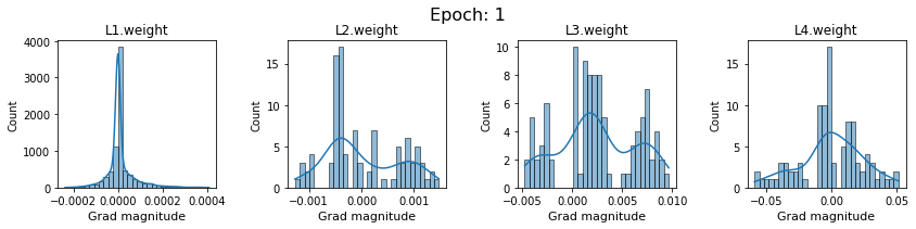
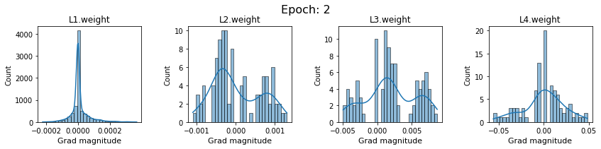
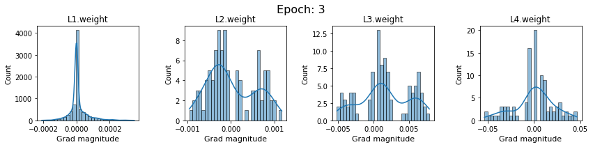
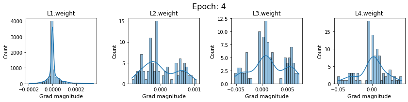
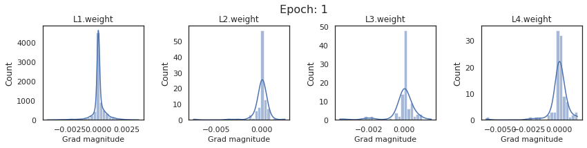
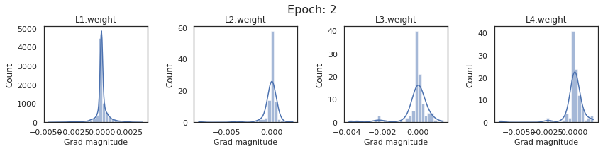
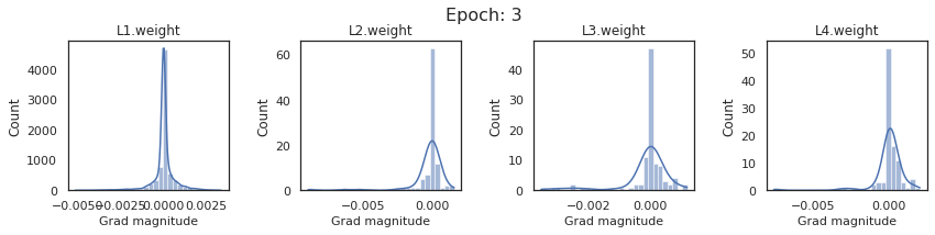
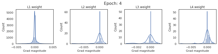
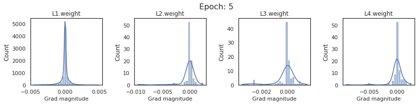
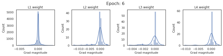
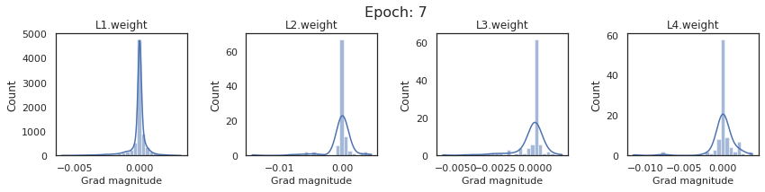
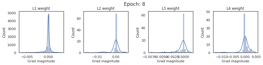
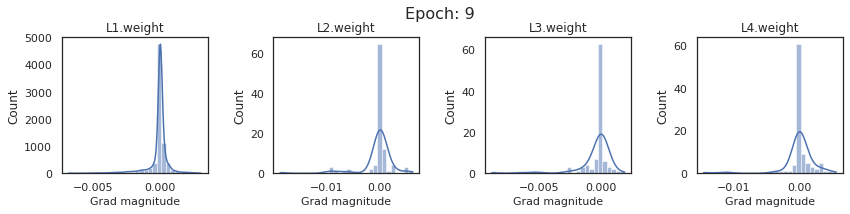
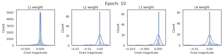
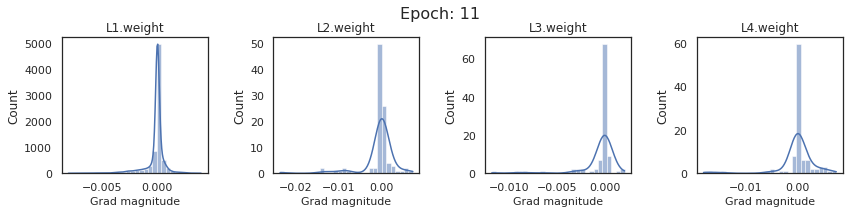
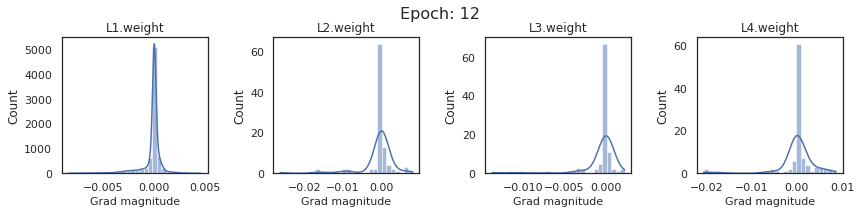
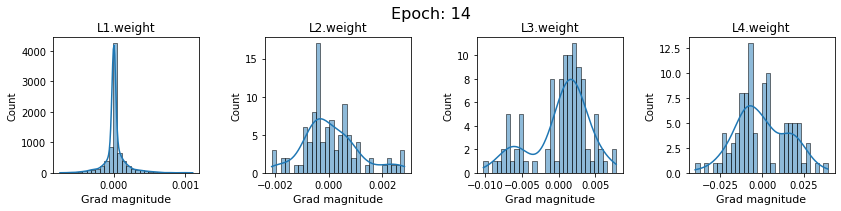
    plt.close()

Plot the gradients for model with sigmoid activations.

for i in range(len(dlp_sigmoid.grad)):
    plot_gradients(dlp_sigmoid.grad[i], i)

What do we get from these plots?

Issues

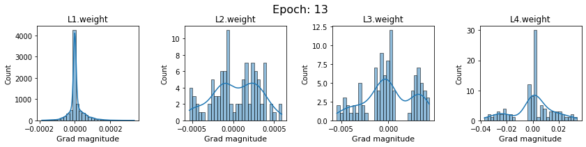
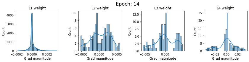
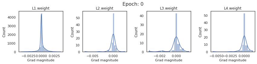
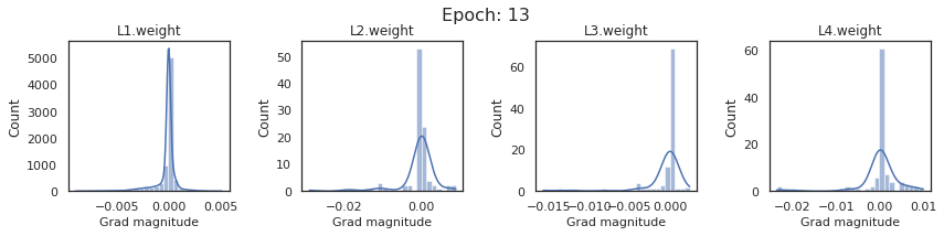
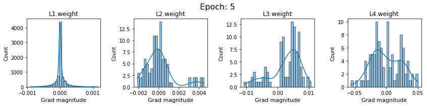
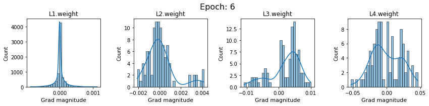
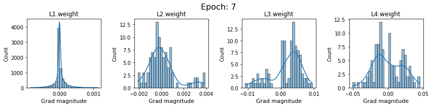
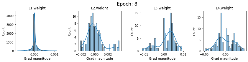
In this section, we will discuss the issues we can identify from these gradient plots for our SigmoidNet

Issue 1: Look closely at how the Grad magnitude scale changes from L4 to L1 in an epoch. It is diminishing at an exponential rate. This tells us that the gradient is very high at the output layer but diminishes till it reaches L1.

Issue 2: Gradient is also spread out and not smoother. This is a bad sign because it shows that different areas of the weight layer produce gradients in different ranges. For example, from L4 plot in the last epoch, we can see that the gradients are making clusters around -0.02, 0, and 0.02. We can also find that the gradient mean is not centered around 0. Either it is on the left of 0, or right, or has multiple peaks.

Possible explanations

Issue 1 Reason: Our network is facing Diminishing Gradient problem. I have pasted below another plot for Sigmoid. Image source

sigmoid.png

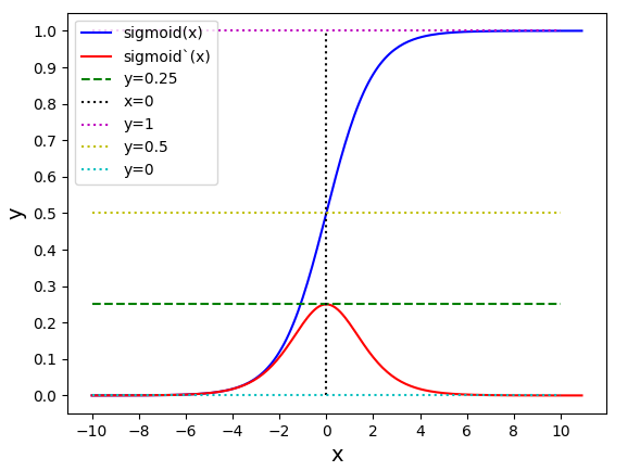
From this plot, we can see that the highest gradient produced by sigmoid is 0.25. So during backpropagation, when we calculate derivatives for deeper layers (L1, L2), there is a chain reaction where smaller and smaller numbers (less than 0.25) are multiplied to produce even smaller numbers. The result is that gradients diminish, and the weights are barely updated in deeper layers during the backward pass. We can avoid this by using a different activation function (e.g., ReLU) in hidden layers. We will do that in Section II.

Issue 2 Reason: This is due to an initial weight initialization mismatch with the activation function used. By default, PyTorch uses kaiming initialization (Ref here) that works well for ReLU but not for sigmoid. It’s recommended to use Tanh or Xavior for sigmoid.

Can we improve our SigmoidNet?

Let’s train another SigmoidNet with the same configuration but with xavior initialization , and observe how it behaves now.

#collapse-output
model_sigmoid_v1 = SigmoidNet
model_sigmoid_v1 = model_sigmoid_v1.to(device)

# define a function to initialize weight with xavier uniform distribution
def init_weights(m):
    if isinstance(m, nn.Linear):
        torch.nn.init.xavier_uniform_(m.weight)
        # m.bias.data.fill_(0.01)

# reset model weights with xavier
with torch.no_grad():
    model_sigmoid_v1.apply(init_weights)

lr = 0.001
optimizer_sigmoid = optim.SGD(model_sigmoid_v1.parameters(), lr=lr)
loss_fn = nn.CrossEntropyLoss()

n_epochs = 15

dlp_sigmoid_v1 = DeepLearningPipeline(model_sigmoid_v1, loss_fn, optimizer_sigmoid)
dlp_sigmoid_v1.set_loaders(train_loader, valid_loader)
dlp_sigmoid_v1.train(n_epochs)

epoch:   0, train loss: 2.49727, valid loss: 2.45576
epoch:   1, train loss: 2.46252, valid loss: 2.42681
epoch:   2, train loss: 2.43418, valid loss: 2.40356
epoch:   3, train loss: 2.41090, valid loss: 2.38474
epoch:   4, train loss: 2.39164, valid loss: 2.36943
epoch:   5, train loss: 2.37565, valid loss: 2.35693
epoch:   6, train loss: 2.36232, valid loss: 2.34670
epoch:   7, train loss: 2.35119, valid loss: 2.33831
epoch:   8, train loss: 2.34186, valid loss: 2.33143
epoch:   9, train loss: 2.33404, valid loss: 2.32578
epoch:  10, train loss: 2.32746, valid loss: 2.32113
epoch:  11, train loss: 2.32192, valid loss: 2.31731
epoch:  12, train loss: 2.31724, valid loss: 2.31417
epoch:  13, train loss: 2.31328, valid loss: 2.31159
epoch:  14, train loss: 2.30993, valid loss: 2.30946

fig = dlp_sigmoid_v1.plot_losses()

##
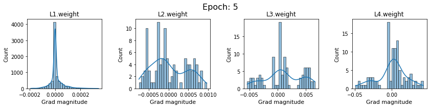
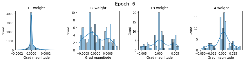
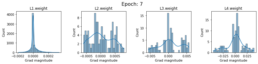
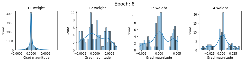
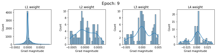
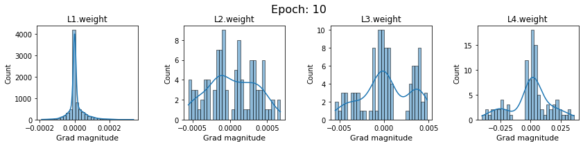
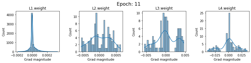
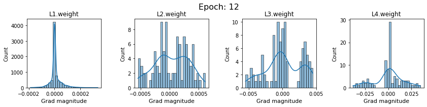
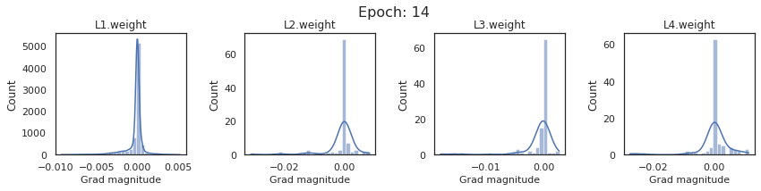
#  SigmoidNet gradients with xavior initialization
for i in range(len(dlp_sigmoid_v1.grad)):
    plot_gradients(dlp_sigmoid_v1.grad[i], i)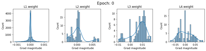

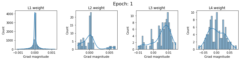
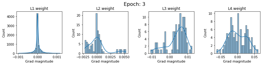
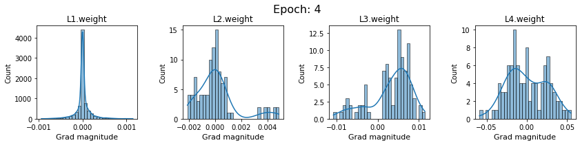
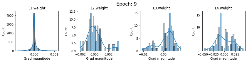
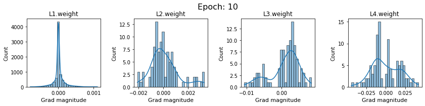
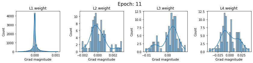
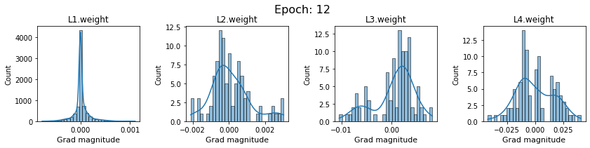
Now the plots are much smoother. Though the network is still suffering from diminishing gradients.

Ridge plot for gradients

In this section, we will use ridge plots for gradients. They provide a better perspective on how gradients evolve during epochs.

Code

import pandas as pd

# A helper function to get gradients of a weight layer for all epochs.
def get_layer_gradients(layer_name, layer_grads):
    df = pd.DataFrame(columns=['x','g'])
    for i in range(len(layer_grads)):
        temp = {
            'x': layer_grads[i][layer_name], # x --> gradients
            'g': i # g --> epochs
        }
        epoch_df = pd.DataFrame(temp)
        df = df.append(epoch_df, ignore_index=True)

    return df

Print the names for the model weight layers.

weight_layers_sigmoid_v1 = list(dlp_sigmoid_v1.grad[0].keys())
weight_layers_sigmoid_v1

['L1.weight', 'L2.weight', 'L3.weight', 'L4.weight']

Store the gradients for each layer in a separate DataFrame. Each DataFrame has two columns

• x: for the gradient value
• g: for epoch

df0_sigmoid_v1 = get_layer_gradients(weight_layers_sigmoid_v1[0], dlp_sigmoid_v1.grad)
df1_sigmoid_v1 = get_layer_gradients(weight_layers_sigmoid_v1[1], dlp_sigmoid_v1.grad)
df2_sigmoid_v1 = get_layer_gradients(weight_layers_sigmoid_v1[2], dlp_sigmoid_v1.grad)
df3_sigmoid_v1 = get_layer_gradients(weight_layers_sigmoid_v1[3], dlp_sigmoid_v1.grad)

df3_sigmoid_v1.head()

	x	g
0	-0.003590	0
1	-0.002747	0
2	-0.002291	0
3	-0.006168	0
4	-0.002711	0

Code

# Another helper function to create the ridge plots
def plot_gradients_ridge_v1(df, layer_name):
    sns.set_theme(style="white", rc={"axes.facecolor": (0, 0, 0, 0)})

    # Initialize the FacetGrid object
    pal = sns.cubehelix_palette(10, rot=-.25, light=.7)
    g = sns.FacetGrid(df, row="g", hue="g", aspect=15, height=.5, palette=pal)

    # Draw the densities in a few steps
    g.map(sns.kdeplot, "x",
        bw_adjust=.5, clip_on=False,
        fill=True, alpha=1, linewidth=1.5)
    g.map(sns.kdeplot, "x", clip_on=False, color="w", lw=2, bw_adjust=.5)

    # passing color=None to refline() uses the hue mapping
    g.refline(y=0, linewidth=2, linestyle="-", color=None, clip_on=False)


    # Define and use a simple function to label the plot in axes coordinates
    def label(x, color, label):
        ax = plt.gca()
        ax.text(0, .2, label, fontweight="bold", color=color,
                ha="left", va="center", transform=ax.transAxes)


    g.map(label, "x")

    # Set the subplots to overlap
    g.figure.subplots_adjust(hspace=-.25)

    g.fig.suptitle(layer_name, ha='left', fontsize=16, fontweight=16)

    # Remove axes details that don't play well with overlap
    g.set_titles("")
    g.set(yticks=[], ylabel="")
    g.despine(bottom=True, left=True)

    return g

Create plots for all weight layer.

Code

# https://stackoverflow.com/questions/35042255/how-to-plot-multiple-seaborn-jointplot-in-subplot
import warnings
import matplotlib.image as mpimg
warnings.filterwarnings("ignore")

g1 = plot_gradients_ridge_v1(df0_sigmoid_v1, weight_layers_sigmoid_v1[0])
g2 = plot_gradients_ridge_v1(df1_sigmoid_v1, weight_layers_sigmoid_v1[1])
g3 = plot_gradients_ridge_v1(df2_sigmoid_v1, weight_layers_sigmoid_v1[2])
g4 = plot_gradients_ridge_v1(df3_sigmoid_v1, weight_layers_sigmoid_v1[3])

g1.savefig('g1.png')
plt.close(g1.fig)

g2.savefig('g2.png')
plt.close(g2.fig)

g3.savefig('g3.png')
plt.close(g3.fig)

g4.savefig('g4.png')
plt.close(g4.fig)

############### 3. CREATE YOUR SUBPLOTS FROM TEMPORAL IMAGES
f, axarr = plt.subplots(2, 2, figsize=(25, 16))

axarr[0,0].imshow(mpimg.imread('g1.png'))
axarr[0,1].imshow(mpimg.imread('g2.png'))
axarr[1,0].imshow(mpimg.imread('g3.png'))
axarr[1,1].imshow(mpimg.imread('g4.png'))


# turn off x and y axis
[ax.set_axis_off() for ax in axarr.ravel()]

plt.tight_layout()
plt.show()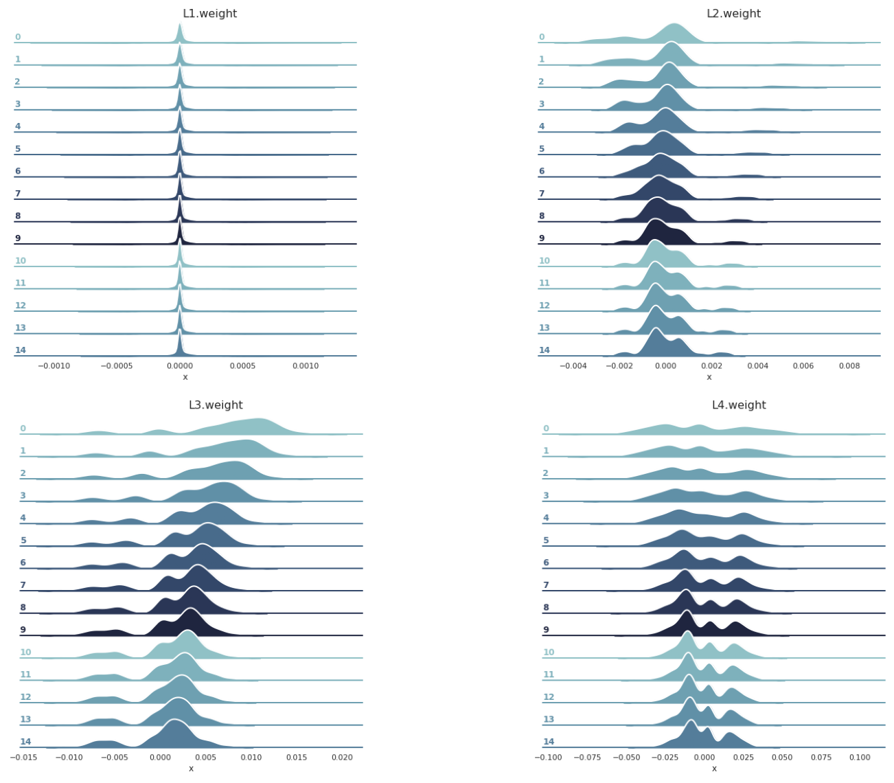

What do we get from these ridge plots?

• It also shows that the network is suffering from diminishing gradients. gradient scale ‘x’ is decreasing exponentially between weight layers
• It shows that gradients are very spread out at the start. They keep on saturating till around epoch 10. After that, instead of getting more saturated around zero, multiple peaks start to emerge. This could be due to our learning rate. In the later epochs, our weights start to oscillate around zero. We can avoid this by using an adaptive learning rate that decreases when weights are near the global minimum.

Gradients for a model with ReLU activations

In this section we will visualize gradients for our model with ReLU activations.

for i in range(len(dlp_relu.grad)):
    plot_gradients(dlp_relu.grad[i], i)

What do we get from these plots?

• This time, the gradient curves are nice and smooth. They are not diminishing between weight layers.
• Gradients are shrinking between epochs. This means that learning is slowing down in later epochs, and we need to increase the learning rate.

Ridge plot for gradients

Let’s also do ridge plots for ReluNet.

Code

# a helper function relu ridge plots. 
# same as 'plot_gradients_ridge_v1' but with added limits
def plot_gradients_ridge_v2(df, layer_name):
    sns.set_theme(style="white", rc={"axes.facecolor": (0, 0, 0, 0)})

    # Initialize the FacetGrid object
    pal = sns.cubehelix_palette(10, rot=-.25, light=.7)
    g = sns.FacetGrid(df, row="g", hue="g", aspect=15, height=3.5, palette=pal, sharex=False, xlim=(-0.01,0.01)) ## works best
    # g = sns.FacetGrid(df, row="g", hue="g", aspect=7, height=3.5, palette=pal)#, sharex=False, xlim=(-0.01,0.01)) ## works good

    # Draw the densities in a few steps
    g.map(sns.kdeplot, "x", bw_adjust=.5, clip_on=True, fill=True, alpha=1, linewidth=1.5)
    g.map(sns.kdeplot, "x", clip_on=True, color="w", lw=2, bw_adjust=.5)

    # passing color=None to refline() uses the hue mapping
    g.refline(y=0, linewidth=2, linestyle="-", color=None, clip_on=True)


    # Define and use a simple function to label the plot in axes coordinates
    def label(x, color, label):
        ax = plt.gca()
        ax.text(0, .2, label, fontsize=40, fontweight=26, color=color, ha="left", va="center", transform=ax.transAxes)


    g.map(label, "x")

    # Set the subplots to overlap
    g.figure.subplots_adjust(hspace=-.25)

    g.fig.suptitle(layer_name, ha='left', fontsize=40, fontweight=26)

    # Remove axes details that don't play well with overlap
    g.set_titles("")
    g.set(yticks=[], ylabel="")
    g.despine(bottom=True, left=True)
    plt.xticks(fontsize=35)

    return g

Code

weight_layers_relu = list(dlp_relu.grad[0].keys())

df0_relu = get_layer_gradients(weight_layers_relu[0], dlp_relu.grad)
df1_relu = get_layer_gradients(weight_layers_relu[1], dlp_relu.grad)
df2_relu = get_layer_gradients(weight_layers_relu[2], dlp_relu.grad)
df3_relu = get_layer_gradients(weight_layers_relu[3], dlp_relu.grad)

Code

import matplotlib.image as mpimg
warnings.filterwarnings("ignore")

g1 = plot_gradients_ridge_v2(df0_relu, weight_layers_relu[0])
g2 = plot_gradients_ridge_v2(df1_relu, weight_layers_relu[1])
g3 = plot_gradients_ridge_v2(df2_relu, weight_layers_relu[2])
g4 = plot_gradients_ridge_v2(df3_relu, weight_layers_relu[3])

g1.savefig('g1.png')
plt.close(g1.fig)

g2.savefig('g2.png')
plt.close(g2.fig)

g3.savefig('g3.png')
plt.close(g3.fig)

g4.savefig('g4.png')
plt.close(g4.fig)

############### 3. CREATE YOUR SUBPLOTS FROM TEMPORAL IMAGES
f, axarr = plt.subplots(2, 2, figsize=(25, 16))

axarr[0,0].imshow(mpimg.imread('g1.png'))
axarr[0,1].imshow(mpimg.imread('g2.png'))
axarr[1,0].imshow(mpimg.imread('g3.png'))
axarr[1,1].imshow(mpimg.imread('g4.png'))


# turn off x and y axis
[ax.set_axis_off() for ax in axarr.ravel()]

plt.tight_layout()
plt.show()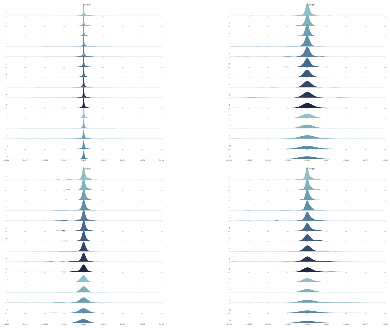

What do we get from these ridge plots?

The results are consistent with earlier plots.

• Gradients are not diminishing between weight layers.
• Gradients are shrinking between epochs, and we need to increase the learning rate for later epochs.